Business Report Analysis: Forecasting Methods and Solutions

This report presents an analysis of a business report, focusing on forecasting methods and their application. It begins with an analysis of a production plan, including the optimal values of an objective function, production quantities for SUVs and cars across four quarters, and a sensitivity report. The sensitivity report highlights the impact of changes in production on the objective function, including allowable increases and decreases for various variables. The report then delves into forecasting methods, differentiating between qualitative and quantitative approaches and emphasizing the use of time series data. It outlines the autoregressive moving average (ARMA) model, the Box-Jenkins approach, and the importance of data stationarity and diagnostic checking. The report references various sources to support its findings, including studies on time series forecasting, hybrid models, and economic analysis. The report concludes that the company should consider persuading the government to relax the mpg requirement, as this will be beneficial since more SUV can be produced in all quarter and more cars allowed in quarter 1 and 3 since a change in one unit has a significant change in the optimal value of the objective function.

1. Report analysis for jakes
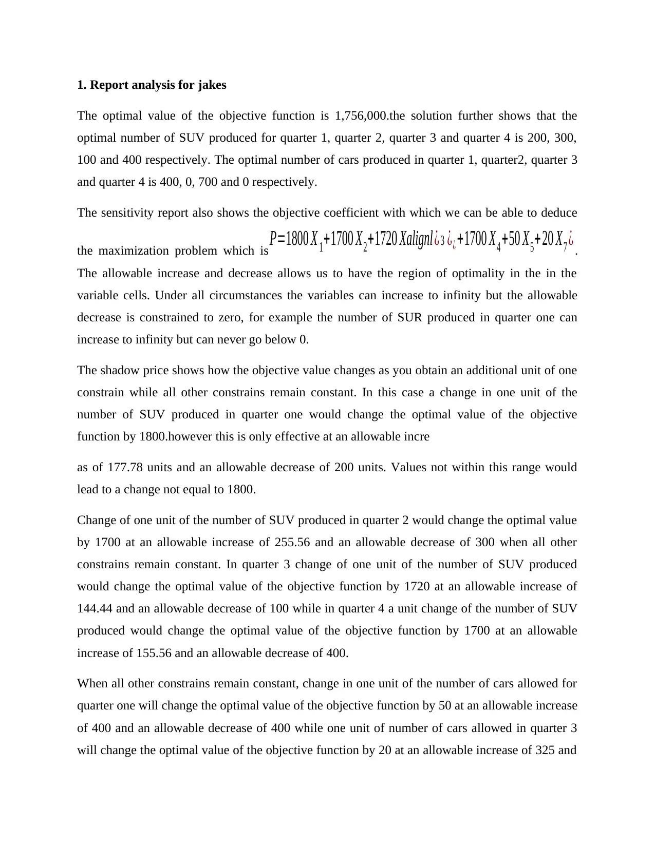
The optimal value of the objective function is 1,756,000.the solution further shows that the
optimal number of SUV produced for quarter 1, quarter 2, quarter 3 and quarter 4 is 200, 300,
100 and 400 respectively. The optimal number of cars produced in quarter 1, quarter2, quarter 3
and quarter 4 is 400, 0, 700 and 0 respectively.
The sensitivity report also shows the objective coefficient with which we can be able to deduce
the maximization problem which is P=1800 X 1+1700 X2+1720 Xalignl ¿ 3 ¿¿ +1700 X4 +50 X5+ 20 X7 ¿ .
The allowable increase and decrease allows us to have the region of optimality in the in the
variable cells. Under all circumstances the variables can increase to infinity but the allowable
decrease is constrained to zero, for example the number of SUR produced in quarter one can
increase to infinity but can never go below 0.
The shadow price shows how the objective value changes as you obtain an additional unit of one
constrain while all other constrains remain constant. In this case a change in one unit of the
number of SUV produced in quarter one would change the optimal value of the objective
function by 1800.however this is only effective at an allowable incre
as of 177.78 units and an allowable decrease of 200 units. Values not within this range would
lead to a change not equal to 1800.
Change of one unit of the number of SUV produced in quarter 2 would change the optimal value
by 1700 at an allowable increase of 255.56 and an allowable decrease of 300 when all other
constrains remain constant. In quarter 3 change of one unit of the number of SUV produced
would change the optimal value of the objective function by 1720 at an allowable increase of
144.44 and an allowable decrease of 100 while in quarter 4 a unit change of the number of SUV
produced would change the optimal value of the objective function by 1700 at an allowable
increase of 155.56 and an allowable decrease of 400.
When all other constrains remain constant, change in one unit of the number of cars allowed for
quarter one will change the optimal value of the objective function by 50 at an allowable increase
of 400 and an allowable decrease of 400 while one unit of number of cars allowed in quarter 3
will change the optimal value of the objective function by 20 at an allowable increase of 325 and

an allowable decrease of 700. Change in one unit of the number of cars allowed in quarter 2 and
quarter 4 has no effect on the optimal value of the objective function.
The company should consider persuading the regional government to relax the mpg requirement
as this will be beneficial since more SUV can be produced in all quarter and more cars allowed
in quarter 1 and 3 since a change in one unit has a significant change in the optimal value of the
objective function.
Fall in the profit contribution of SUV would heavily affect the production plan since it’s the
main contributor to the net profit.
2.
Forecasting method mainly depend on what data are available. The main types of forecast are
qualitative and quantitative forecasting. In the absence of past observation qualitative method of
forecasting must be used. Quantitative method on the other hand is used when past numerical
information is available and under the reasonable assumption that past patterns will continue in
the future.
In this data time series data shall be used since the observation are collected over a regular
interval of time. Time series forecast is useful when forecasting something that is changing over
time for example the stock market, monthly rainfall, quarterly sales of companies and profit.
The aim of forecasting is time series data is to estimate how the sequence of the visitors will
continue into the future. We shall only use the information on the variable to be forecasted which
is visitors but shall not explain the factors that cause the behavior.
The main linear model used includes the autoregressive process (AR), the moving average (MA)
and the autoregressive moving average (ARMA). The ARMA model is a statistical technique
that uses the series data to predict the future parameters used. An ARMA model takes care of
trend, seasonality, errors and non-stationary aspect of data when forecasting. In order to apply
the models, any deterministic trends or cycles must be removed. The data provided should first
be checked if it is stationary or non-stationary. If stationary differencing should be used This can

be achieved by plotting the autocorrelation function (ACF) and partial autocorrelation function
(PACF) graphs.
The ACF calculates the correlation at different lag interval to help identify any dependence
within the data. If lags in the ACF exceed the confidence interval the process is non-stationary,
and thus is used in the ARIMA model to capture dependent lags with high autocorrelation.
The model with the smallest possible number of parameters is to be selected so as to provide
adequate and sufficient representation of the underlying time series data. This ensures it is
suitable for future forecasting as over fitting affect the ability of a model to forecast well.
After the tentative identification of an ARIMA (p, qi) model and calculation of the estimates we
have to perform diagnostic checking. The principle of this is that, if the ARMA (p, q) model is a
good approximation to the underlying time series process, then the residuals will form a good
approximation to a white noise process.
Box –Jenkins approach to forecasting stationary time series should be used to forecast number of
visitors for the coming year.
This resulting stationary series can then be modeled by a stationary ARMA (p,q)process. The
values p and q are first determined by looking at the sample autocorrelation and sample partial
autocorrelation functions. If differences were required to make the series stationary, then the
original series will be modeled by an ARIMA (p,d,q) process. The calibration of the model, that
is finding the parameter values, is carried out in much the same way as linear regression is done
in
Once a potential model has been found then a series of diagnostic tests on the residuals can be
applied to check its validity. In contrast to modeling in terms of mathematical equation, the
moving average rarely smooths the fluctuation in the data. A moving average works well when
the data have a fairly linear trend and a definite pattern of fluctuation.

References:
1. A Parashar, “Impact analysis of distributed generation and RE based distributed generation on
Indian economy and economy of Bop”, available on
www.wipro.org/earthian/documents/1000925_IITKGP_REPaper.pdf.
2. Brockwell, P. J. and R. A. Davis. Introduction to Time Series and Forecasting. 2nd ed. New
York, NY: Springer, 2002.
3 E. S. Hrayshat, “Techno-Economic Analysis of Autonomous Hybrid Photovoltaic-Diesel-
Battery System,” Energy for Sustainable Development, Vol. 13, No. 3, 2009, pp. 143-150.
doi:10.1016/j.esd.2009.07.003
4. G.P. Zhang, “Time series forecasting using a hybrid ARIMA and neural network model”,
Neurocomputing 50 (2003), pages: 159–175.
5. J. L. Bernal-Agustin and R. Dufo-Lopez, “Economical and Environmental Analysis of Grid
Connected Photo- voltaic Systems in Spain,” Renewable Energy, Vol. 31, No. 8, 2006, pp.
1107-1128. doi:10.1016/j.renene.2005.06.004.
6. J. Faraway, C. Chatfield, “Time series forecasting with neural networks: a comparative study
using the airline data”, Applied Statistics 47 (1998), pages: 231–250
7. J. Lee, “Univariate time series modeling and forecasting (Box-Jenkins Method)”, Econ 413,
lecture 4.
8. J.M. Kihoro, R.O. Otieno, C. Wafula, “Seasonal Time Series Forecasting: A Comparative
Study of ARIMA and ANN Models”, African Journal of Science and Technology (AJST)
Science and Engineering Series Vol. 5, No. 2, pages: 41-49
9. Neter, John, William Wasserman, and Michael H. Kutner. Applied Linear Statistical Models.
Homewood, IL: Irwin, 1990. Print.
10. P.G. Zhang, “Time series forecasting using a hybrid ARIMA and neural network model”,
Neurocomputing 50 (2003), pages: 159–175