Business Modelling for Decision Making: Inventory, Profit, and Tree
VerifiedAdded on 2022/12/28
|14
|3187
|1
Report
AI Summary
This report delves into business modelling as a crucial aspect of business, enabling effective exploration of complex choices through various assumptions. It covers inventory management, non-linear/extremum problems, and decision tree analysis. Part A focuses on inventory, calculating EOQ for A545 Plasma TVs, determining optimal deliveries, and computing total annual variable costs. Part B explores non-linear/extremum analysis, creating a profit equation for a London furniture maker, setting up demand, costs, and profit tables, and differentiating the profit equation to maximize profit. Part C involves constructing and analyzing a decision tree based on a case study. The report concludes by highlighting the importance of business modelling in achieving organizational objectives and ensuring sustainability.
Business Modelling for
Decision Making
Decision Making
Paraphrase This Document
Need a fresh take? Get an instant paraphrase of this document with our AI Paraphraser
Contents
INTRODUCTION................................................................................................................................3
MAIN BODY......................................................................................................................................3
Part A – INVENTORY.........................................................................................................................3
(a). Computation of EOQ (economic-order quantity) with respect to A545 Plasma TV, applying
specific formula:...........................................................................................................................3
(b). On the basis of above computed EOQ level assessing how much quantities/deliveries
should be made of A545 Plasma TVs per year:............................................................................3
(c). Find the total annual variable cost for TV King Ltd:...............................................................4
(d).................................................................................................................................................4
(e).................................................................................................................................................4
Part B – NON-LINEAR/EXTREMUM..................................................................................................7
a) Finding out an equation with respect to profit level of London furniture makers:................7
b) Setting up demand, costs and profit table...............................................................................8
c) Using values from above stated table and drawing a demand, costs and profitability graph 8
(d). Based on above displayed graph, differentiating profit level equation to assess actual
value of ‘q’ where profit level maximises:...................................................................................9
e) Assessing value of ‘X’ coefficients dependent on q (Liverpool):..............................................9
f. Strong and weak points in the London and Liverpool models:................................................9
Part C – DECISION TREE.................................................................................................................10
SECTION 1...................................................................................................................................10
i...................................................................................................................................................10
ii. Decision Tree:.........................................................................................................................12
SECTION 2...................................................................................................................................12
CONCLUSION..................................................................................................................................13
REFERENCES...................................................................................................................................14
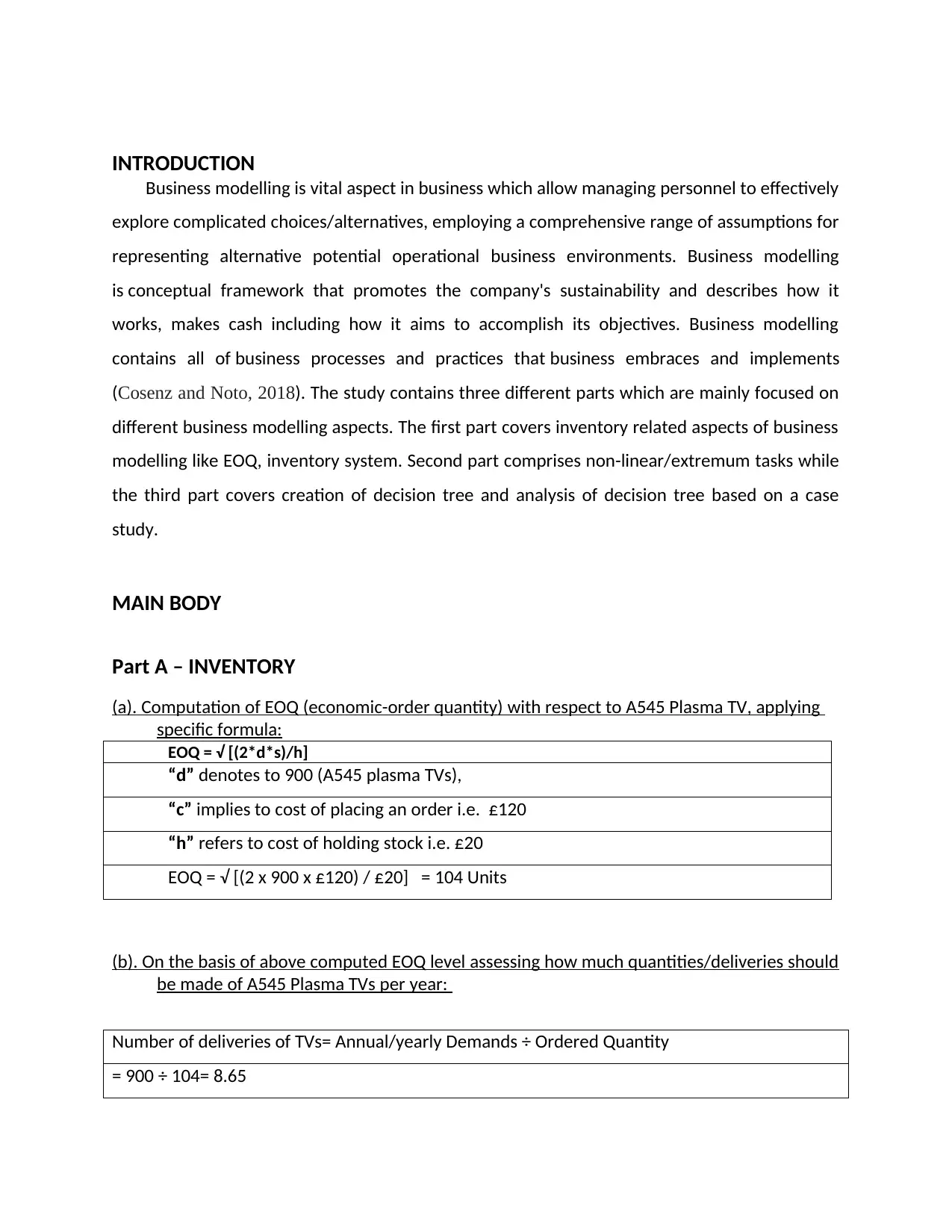
INTRODUCTION
Business modelling is vital aspect in business which allow managing personnel to effectively
explore complicated choices/alternatives, employing a comprehensive range of assumptions for
representing alternative potential operational business environments. Business modelling
is conceptual framework that promotes the company's sustainability and describes how it
works, makes cash including how it aims to accomplish its objectives. Business modelling
contains all of business processes and practices that business embraces and implements
(Cosenz and Noto, 2018). The study contains three different parts which are mainly focused on
different business modelling aspects. The first part covers inventory related aspects of business
modelling like EOQ, inventory system. Second part comprises non-linear/extremum tasks while
the third part covers creation of decision tree and analysis of decision tree based on a case
study.
MAIN BODY
Part A – INVENTORY
(a). Computation of EOQ (economic-order quantity) with respect to A545 Plasma TV, applying
specific formula:
EOQ = √ [(2*d*s)/h]
“d” denotes to 900 (A545 plasma TVs),
“c” implies to cost of placing an order i.e. £120
“h” refers to cost of holding stock i.e. £20
EOQ = √ [(2 x 900 x £120) / £20] = 104 Units
(b). On the basis of above computed EOQ level assessing how much quantities/deliveries should
be made of A545 Plasma TVs per year:
Number of deliveries of TVs= Annual/yearly Demands ÷ Ordered Quantity
= 900 ÷ 104= 8.65
⊘ This is a preview!⊘
Do you want full access?
Subscribe today to unlock all pages.
Trusted by 1+ million students worldwide
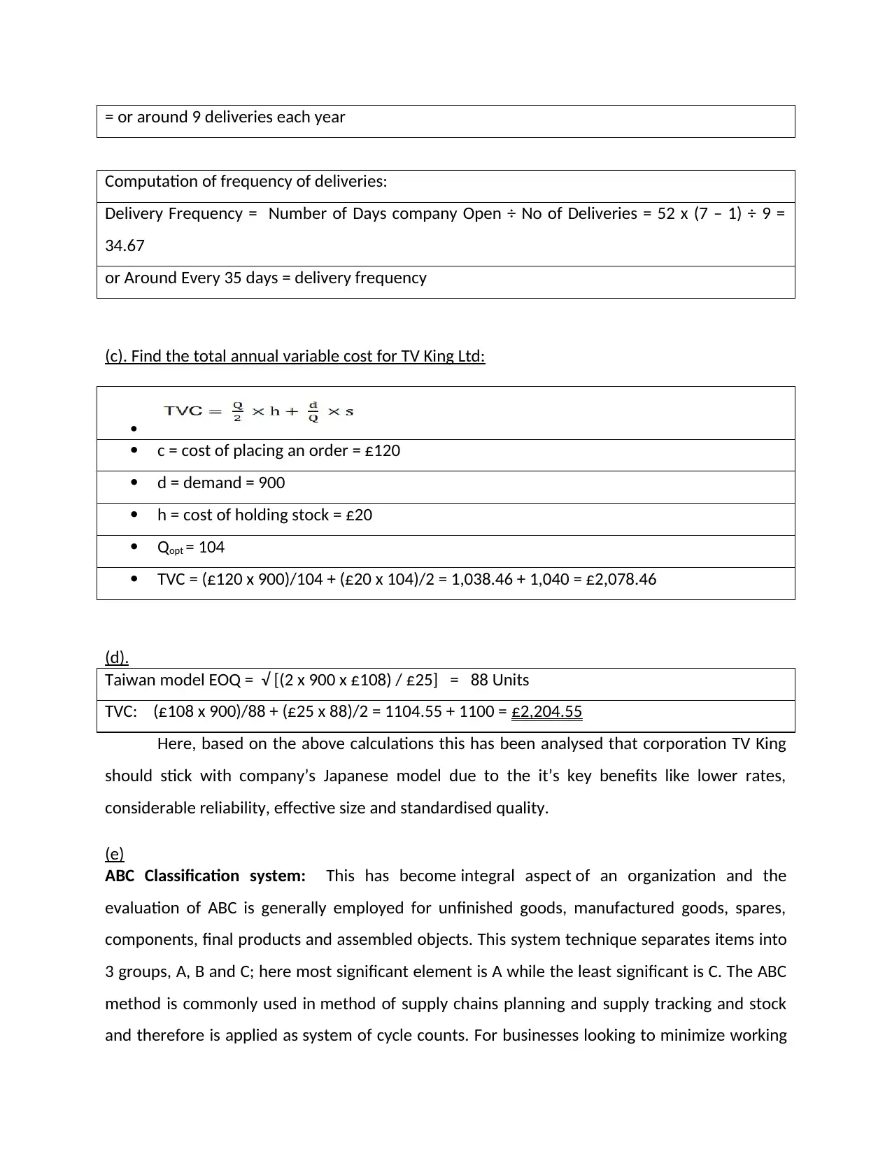
= or around 9 deliveries each year
Computation of frequency of deliveries:
Delivery Frequency = Number of Days company Open ÷ No of Deliveries = 52 x (7 – 1) ÷ 9 =
34.67
or Around Every 35 days = delivery frequency
(c). Find the total annual variable cost for TV King Ltd:
c = cost of placing an order = £120
d = demand = 900
h = cost of holding stock = £20
Qopt = 104
TVC = (£120 x 900)/104 + (£20 x 104)/2 = 1,038.46 + 1,040 = £2,078.46
(d).
Taiwan model EOQ = √ [(2 x 900 x £108) / £25] = 88 Units
TVC: (£108 x 900)/88 + (£25 x 88)/2 = 1104.55 + 1100 = £2,204.55
Here, based on the above calculations this has been analysed that corporation TV King
should stick with company’s Japanese model due to the it’s key benefits like lower rates,
considerable reliability, effective size and standardised quality.
(e)
ABC Classification system: This has become integral aspect of an organization and the
evaluation of ABC is generally employed for unfinished goods, manufactured goods, spares,
components, final products and assembled objects. This system technique separates items into
3 groups, A, B and C; here most significant element is A while the least significant is C. The ABC
method is commonly used in method of supply chains planning and supply tracking and stock
and therefore is applied as system of cycle counts. For businesses looking to minimize working
Paraphrase This Document
Need a fresh take? Get an instant paraphrase of this document with our AI Paraphraser
capital and carrying expenses, this is most essential. This is achieved by reviewing the inventory
which is in surplus inventory as well as those which are outdated by making room for readily
sales made. Instead of keeping it locked up in unsafe stock, this allows to prevent
keeping working capital accessible for use. This allows them to retain control over value
of assets kept at single time if a business is better equipped to monitor the inventory and retain
controlling over high-value products. It also adds order to process of reordering as well as
ensuring that such items are really in inventory to fulfil the requirements. Items falling within
class C are sluggish items which do not need to be re-ordered at same regularity as the items A
or items B (HR and Aithal, 2020). If one brings the products into such three categories,
recognizing the ones that require to be kept and those which could be replaced is useful
for wholesalers as well as distributors. This approach helps corporations retain leverage of
expensive goods that have vast sums of capital investing in them. This offers a means of
keeping control over all inventory for the madness. This not only eliminates excessive payroll
costs, but also ensures that optimal inventory levels are preserved at all stages. The ABC
approach ensures that the inventory turnover rate is sustained at relatively greater level by
systematic inventory management. With this method, storage costs are significantly reduced.
There is arrangement to have adequate stocks in C group to be managed without sacrificing
on more relevant products. Following is categories of items classified under this system:
Item A = Extremely important
Item B = Moderately important
Item C = Relatively unimportant
Item A:
Under ABC system of inventory management and controlling, items grouped under class A are
those items which report maximum values with regard to yearly consumptions. This is
considerable that overall top seventy to eighty percentage of overall annual consumption figure
of corporation generated through just around ten to twenty percentage of aggregate inventory
items. Therefore, this is significant to properly prioritize such items.
Item B:
This includes all items which have mid-range consumption values. These generally equivalent to
around 30 percentage of aggregate stock within corporation that accounts around fifteen to
twenty percentage of overall aggregate yearly consumption values.
Item C:
All items classified under this class bear minimum consumption values as well as account for
around lower than five percentage of total annual consumptions value which implies around
fifty percentage of aggregate stock items.
Note: Here, Yearly consumption value = (Annual demand units) × (item cost per unit)
Buffer/Safety Stock: Safety inventory, commonly alluded to buffer stock,
is surplus/additional inventory which a corporation maintains to ensure that anything does not
running out of inventory One can thought of this as inventory just in scenario. Just in scenario
they running out of items on the shelf, this is additional products held. Many businesses have
been buying small quantities of stock on a daily basis after the introduction of just-in-time stock
systems The premise of just-in-time stock is that businesses should get out of all their storage
centres and only order adequate stock for day or fortnight. Often the inventory is distributed
only as much as few times each day. Just-in-time inventory mechanism will not be used by
many businesses because vendors are not near enough or inventory is hard to deliver. A
protection inventory system is used by these businesses. In this stock method firms purchase
more stocks than they intend to sell. The additional inventory is referred to as their stocks of
protection. This means that during busy seasons/peak time business won't running out of stock.
Buffer inventory is good idea for the satisfaction of clients, although it is risky for the cash flow
of business. Clients are still pleased because famous goods never running out of inventory
(Cosenz and Bivona, 2020).
Pipeline inventory: Pipeline inventory corresponds to stock items which have remained to hit
their ultimate destination in shipping chain of the business. Such items are regarded to be
component of inventory of shipping company through their transit before they have been paid
for by the recipient. When a recipient payment for the objects, furthermore, pipeline inventory
stays on inventory list of a recipient, even though such recipient has still not actually received
them. Before being a final commodity for purchasing by a customer, inventory passes through
⊘ This is a preview!⊘
Do you want full access?
Subscribe today to unlock all pages.
Trusted by 1+ million students worldwide
several distinct locations. Products could arrive from several different nations-for example, one
portion of product may come through China as well as another portion of same product may
come through US. Therefore, product which is on their way through one position to others as
this is referred to as pipeline inventory as it's heading back to next stop in pipeline. It might be
on way from large distributor to warehouse where the finished product would be converted, or
it might be on way from warehouse to local distributor.
Inventory system:
The inventory system is comprehensive approach to inventory acquisition, storage and
distribution of both raw resources (parts) and final products. In commercial sense inventory
system assures the appropriate stock, at right levels, in right place, at right moment, at right
price and at right costs. As aspect of entire supply chain, inventory system involves factors like
monitoring and managing orders, managing stock storage, tracking the quantity of merchandise
for delivery, and order processing from manufacturers as well as consumers. There is series of
guidelines and measures that decide and monitor volume of stocks when inventory needs to be
refilled, and also the amount of inventories that should actually be bought. The inventory
system applies to procedures involving the procurement, storage and profitability of products
from manufacturer to customer across the supply chain. Which appears straightforward but in
attempt to maintain an organized and efficient stock, there are several important daily
processes. A satisfactory equilibrium between all the shifting parts of the storage device cannot
be achieved. Combating statistics like this requires a well-considered strategy and framework
structure for the inventory system. Depending on the, company the items they produce, the
policies they want to uphold, and the scope of their operation, it will take many procedures and
mechanisms to keep operations running (Kalloniatis, McLennan-Smith and Roberts, 2020).
Part B – NON-LINEAR/EXTREMUM
a) Finding out an equation with respect to profit level of London furniture makers:
Demand = 200-15q
Revenue = 200q - 15q2(demand * q2)
Paraphrase This Document
Need a fresh take? Get an instant paraphrase of this document with our AI Paraphraser
Total cost = 120- 8q+12q2
Profit = 200q-15q2 – 120+ 8q-12q2
-27q2+208q-120
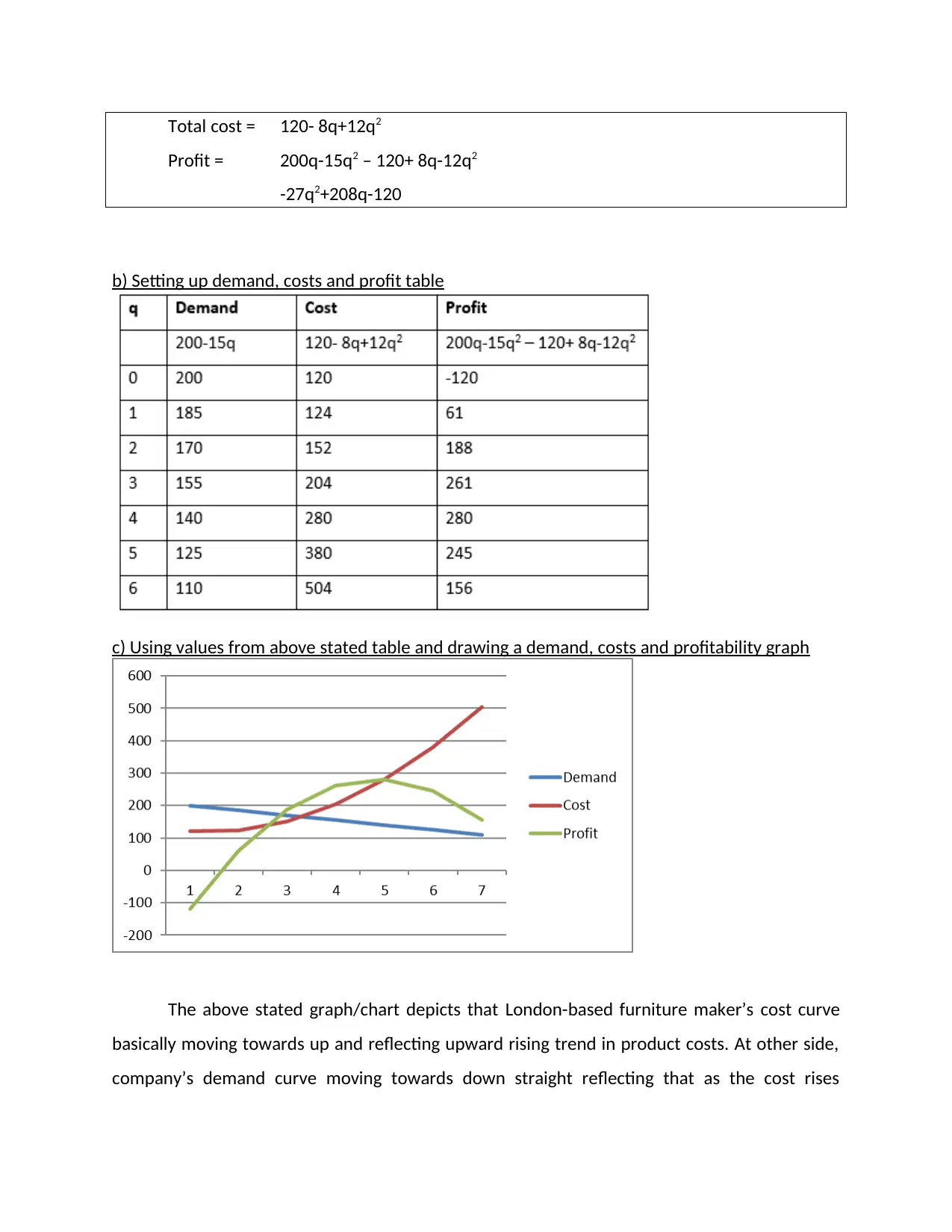
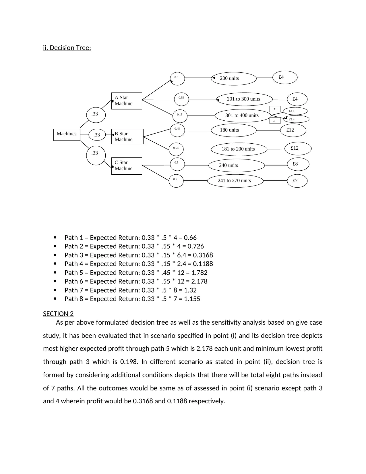
b) Setting up demand, costs and profit table
c) Using values from above stated table and drawing a demand, costs and profitability graph
The above stated graph/chart depicts that London-based furniture maker’s cost curve
basically moving towards up and reflecting upward rising trend in product costs. At other side,
company’s demand curve moving towards down straight reflecting that as the cost rises
Profit = 200q-15q2 – 120+ 8q-12q2
-27q2+208q-120
b) Setting up demand, costs and profit table
c) Using values from above stated table and drawing a demand, costs and profitability graph
The above stated graph/chart depicts that London-based furniture maker’s cost curve
basically moving towards up and reflecting upward rising trend in product costs. At other side,
company’s demand curve moving towards down straight reflecting that as the cost rises
demand for product goes down. Whereas line denoting Profit level goes upward to an extent
then slightly goes downwards which indicates that as the cost rises to 280 profit will decline
along with product demand.
(d). Based on above displayed graph, differentiating profit level equation to assess actual value
of ‘q’ where profit level maximises:
-27q2+208q-120
0 = -54q+208
54q = 208
q = 3.9
e) Assessing value of ‘X’ coefficients dependent on q (Liverpool):
Demand = 200 – 5q
TC = -150 – 25q + 11q2
Profit = -5q2- 11q2+225q – 150
Profit = -16q2 + 225q – 150
(q = 0, 1, 2, 3, 4, 5, 6, 7)
TR – TC =(200q-5q2)-(150-25q+ 11q2)
=200q-5q2-150 + 25q - Xq2
TR – TC =(200q-5q2)-(150-25q+Xq2)
=200q-5q2-150 + 25q - Xq2
= -5q2-Xq2+225q – 150
DERIV: 0 =-10q-2Xq+225
0 =(-10* 5.9) - (2*X*5.9) +225
0 =166 - 11.8X
11.8X = 166
X = 14.1
f. Strong and weak points in the London and Liverpool models:
As per the above performed sensitivity analysis based on the case study of London-based
furniture maker, it has been evaluated that this model for business is quite efficient. Although
there are some key strong merits and demerits. A positive aspect find out within such model is
⊘ This is a preview!⊘
Do you want full access?
Subscribe today to unlock all pages.
Trusted by 1+ million students worldwide
that in business even product demand is overall less but this model enable business to generate
profits. As well as rising costs herein do not directly impact overall profit-level to an extent. On
other hand, demerits of that model is – as demand level increases this model offer decline in
profits and after a certain point even losses.
Moreover, one other demerit of such model asserted is that with decline in overall costs,
business will report decline in overall profit or loss.
Part C – DECISION TREE
SECTION 1
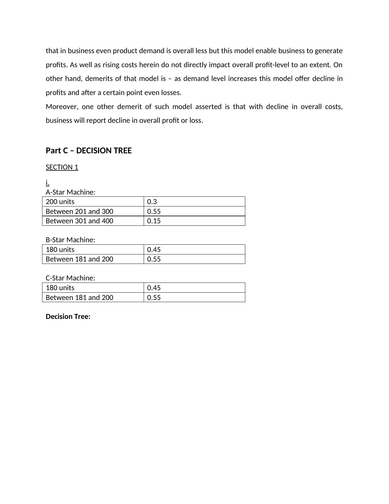
i.
A-Star Machine:
200 units 0.3
Between 201 and 300 0.55
Between 301 and 400 0.15
B-Star Machine:
180 units 0.45
Between 181 and 200 0.55
C-Star Machine:
180 units 0.45
Between 181 and 200 0.55
Decision Tree:
profits. As well as rising costs herein do not directly impact overall profit-level to an extent. On
other hand, demerits of that model is – as demand level increases this model offer decline in
profits and after a certain point even losses.
Moreover, one other demerit of such model asserted is that with decline in overall costs,
business will report decline in overall profit or loss.
Part C – DECISION TREE
SECTION 1
i.
A-Star Machine:
200 units 0.3
Between 201 and 300 0.55
Between 301 and 400 0.15
B-Star Machine:
180 units 0.45
Between 181 and 200 0.55
C-Star Machine:
180 units 0.45
Between 181 and 200 0.55
Decision Tree:
Paraphrase This Document
Need a fresh take? Get an instant paraphrase of this document with our AI Paraphraser
Machines
A Star Machine
B Star Machine
C Star Machine
0.3 200 units
.33
.33
.33
0.55 201 to 300 units
units
0.15 301 to 400 units
0.45
0.55
180 units
181 to 200 units
units
0.5
0.5
240 units
241 to 270 units
Path 1 = Expected Return: 0.33 x .5 x 4 = 0.66
Path 2 = Expected Return: 0.33 x .55 x 4 = 0.726
Path 3 = Expected Return: 0.33 x .15 x 4 = 0.198
Path 4 = Expected Return: 0.33 x .45 x 12 = 1.782
Path 5 = Expected Return: 0.33 x .55 x 12 = 2.178
Path 6 = Expected Return: 0.33 x .5 x 8 = 1.32
Path 7 = Expected Return: 0.33 x .5 x 7 = 1.155
ii. Decision Tree:
Machines
A Star
Machine
B Star
Machine
C Star
Machine
0.3 200 units
.33
.33
.33
0.55 201 to 300 units
units
0.15 301 to 400 units
0.45
0.55
180 units
181 to 200 units
units
0.5
0.5
240 units
241 to 270 units
£4
£4
£6.4
£12
£12
£8
£7
£2.4
.7
.3
Path 1 = Expected Return: 0.33 * .5 * 4 = 0.66
Path 2 = Expected Return: 0.33 * .55 * 4 = 0.726
Path 3 = Expected Return: 0.33 * .15 * 6.4 = 0.3168
Path 4 = Expected Return: 0.33 * .15 * 2.4 = 0.1188
Path 5 = Expected Return: 0.33 * .45 * 12 = 1.782
Path 6 = Expected Return: 0.33 * .55 * 12 = 2.178
Path 7 = Expected Return: 0.33 * .5 * 8 = 1.32
Path 8 = Expected Return: 0.33 * .5 * 7 = 1.155
SECTION 2
As per above formulated decision tree as well as the sensitivity analysis based on give case
study, it has been evaluated that in scenario specified in point (i) and its decision tree depicts
most higher expected profit through path 5 which is 2.178 each unit and minimum lowest profit
through path 3 which is 0.198. In different scenario as stated in point (ii), decision tree is
formed by considering additional conditions depicts that there will be total eight paths instead
of 7 paths. All the outcomes would be same as of assessed in point (i) scenario except path 3
and 4 wherein profit would be 0.3168 and 0.1188 respectively.
⊘ This is a preview!⊘
Do you want full access?
Subscribe today to unlock all pages.
Trusted by 1+ million students worldwide
1 out of 14
Related Documents


Your All-in-One AI-Powered Toolkit for Academic Success.
+13062052269
info@desklib.com
Available 24*7 on WhatsApp / Email
![[object Object]](/_next/static/media/star-bottom.7253800d.svg)
Unlock your academic potential
Copyright © 2020–2026 A2Z Services. All Rights Reserved. Developed and managed by ZUCOL.