Finite Queuing Model Solutions: Business Development Assignment

This document presents a detailed solution to a finite queuing model assignment, focusing on various scenarios and calculations related to service design and queuing theory. The solution covers multiple problems, including analyzing waiting times, calculating costs associated with service improvements, and determining the optimal number of service windows or docks to minimize waiting times and maximize efficiency. It involves applying formulas for arrival and service rates, calculating probabilities, and evaluating the impact of different service configurations on customer waiting times and overall system performance. The document also includes cost-benefit analyses to determine the economic viability of service enhancements, such as installing additional service points or improving existing processes. The analysis considers factors like the average arrival rate, service rate, number of channels, and the resulting impact on waiting times, system utilization, and overall cost savings. The solution provides a comprehensive understanding of queuing models and their application in service design and business development.

Running head: Finite queuing model
Finite queuing model
Student’s name
Institutional affiliation
Date

Finite queuing model 2
Finite queuing model
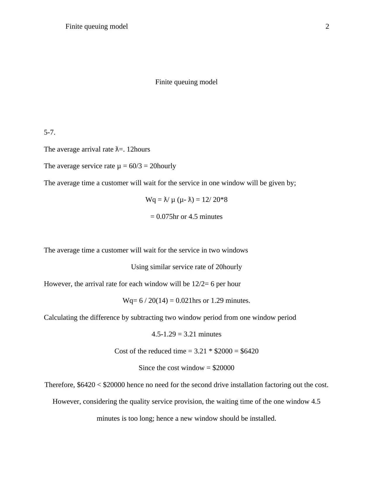
5-7.
The average arrival rate ƛ=. 12hours
The average service rate μ = 60/3 = 20hourly
The average time a customer will wait for the service in one window will be given by;
Wq = ƛ/ μ (μ- ƛ) = 12/ 20*8
= 0.075hr or 4.5 minutes
The average time a customer will wait for the service in two windows
Using similar service rate of 20hourly
However, the arrival rate for each window will be 12/2= 6 per hour
Wq= 6 / 20(14) = 0.021hrs or 1.29 minutes.
Calculating the difference by subtracting two window period from one window period
4.5-1.29 = 3.21 minutes
Cost of the reduced time = 3.21 * $2000 = $6420
Since the cost window = $20000
Therefore, $6420 < $20000 hence no need for the second drive installation factoring out the cost.
However, considering the quality service provision, the waiting time of the one window 4.5
minutes is too long; hence a new window should be installed.

Finite queuing model 3
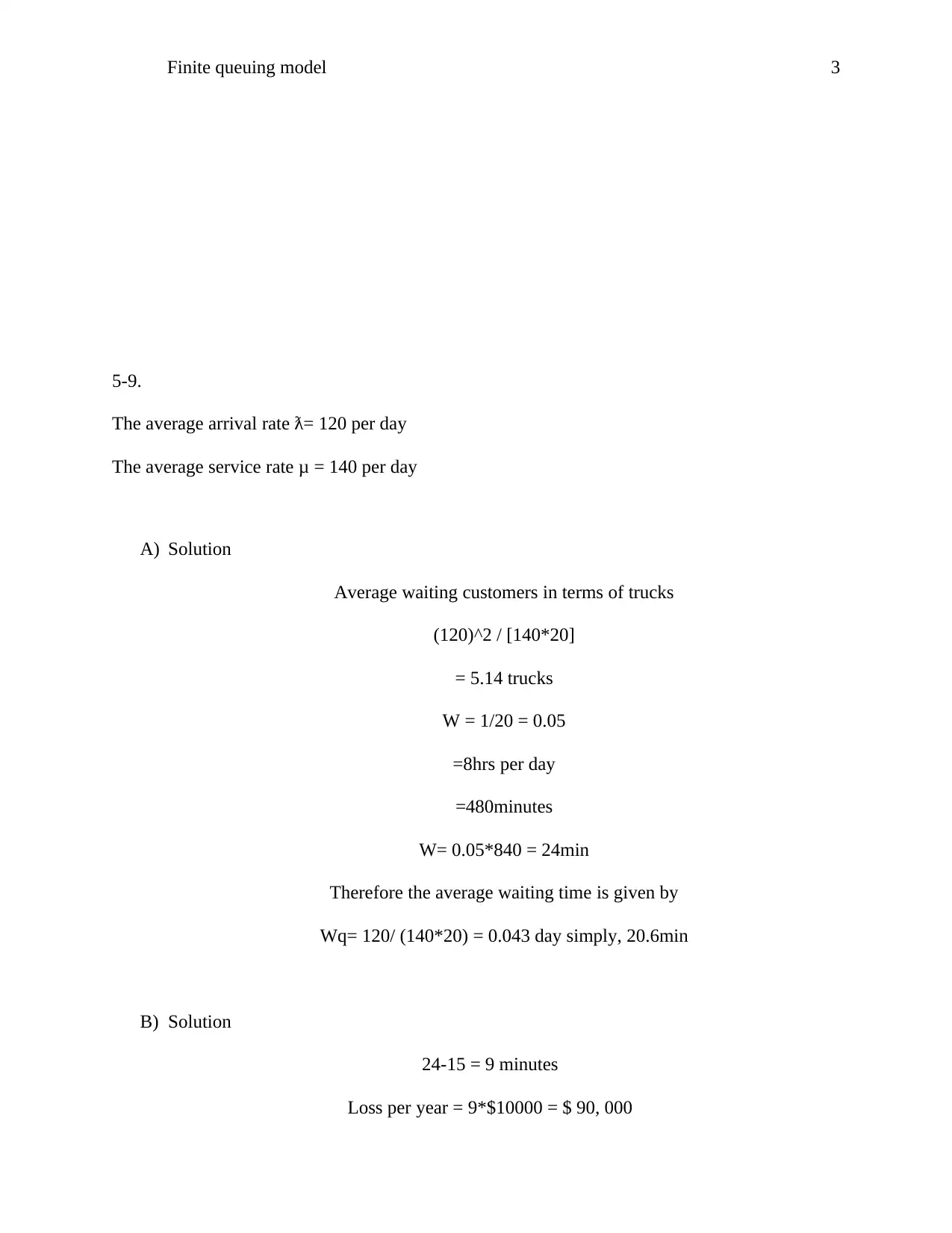
5-9.
The average arrival rate ƛ= 120 per day
The average service rate μ = 140 per day
A) Solution
Average waiting customers in terms of trucks
(120)^2 / [140*20]
= 5.14 trucks
W = 1/20 = 0.05
=8hrs per day
=480minutes
W= 0.05*840 = 24min
Therefore the average waiting time is given by
Wq= 120/ (140*20) = 0.043 day simply, 20.6min
B) Solution
24-15 = 9 minutes
Loss per year = 9*$10000 = $ 90, 000

Finite queuing model 4
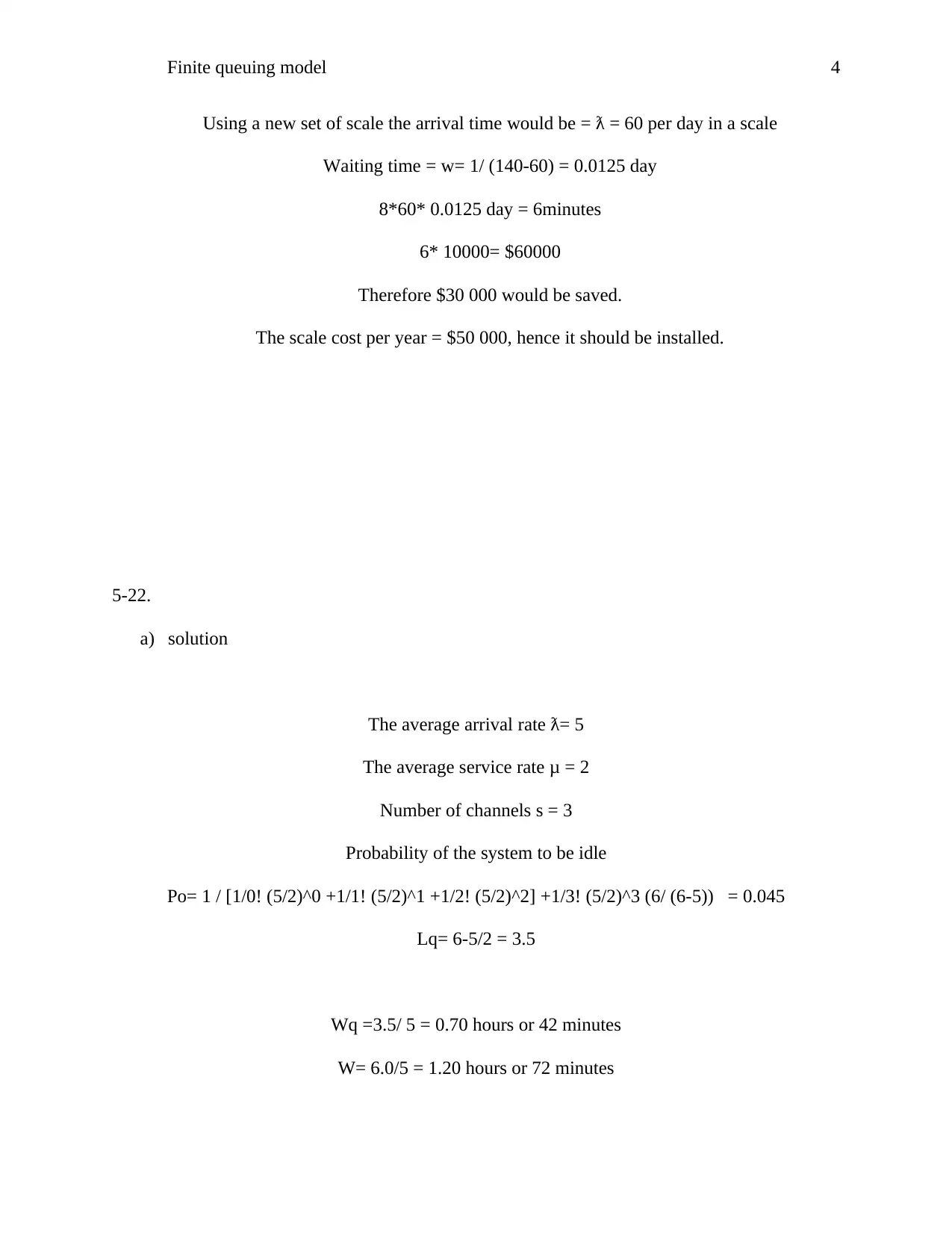
Using a new set of scale the arrival time would be = ƛ = 60 per day in a scale
Waiting time = w= 1/ (140-60) = 0.0125 day
8*60* 0.0125 day = 6minutes
6* 10000= $60000
Therefore $30 000 would be saved.
The scale cost per year = $50 000, hence it should be installed.
5-22.
a) solution
The average arrival rate ƛ= 5
The average service rate μ = 2
Number of channels s = 3
Probability of the system to be idle
Po= 1 / [1/0! (5/2)^0 +1/1! (5/2)^1 +1/2! (5/2)^2] +1/3! (5/2)^3 (6/ (6-5)) = 0.045
Lq= 6-5/2 = 3.5
Wq =3.5/ 5 = 0.70 hours or 42 minutes
W= 6.0/5 = 1.20 hours or 72 minutes

Finite queuing model 5
b) solution
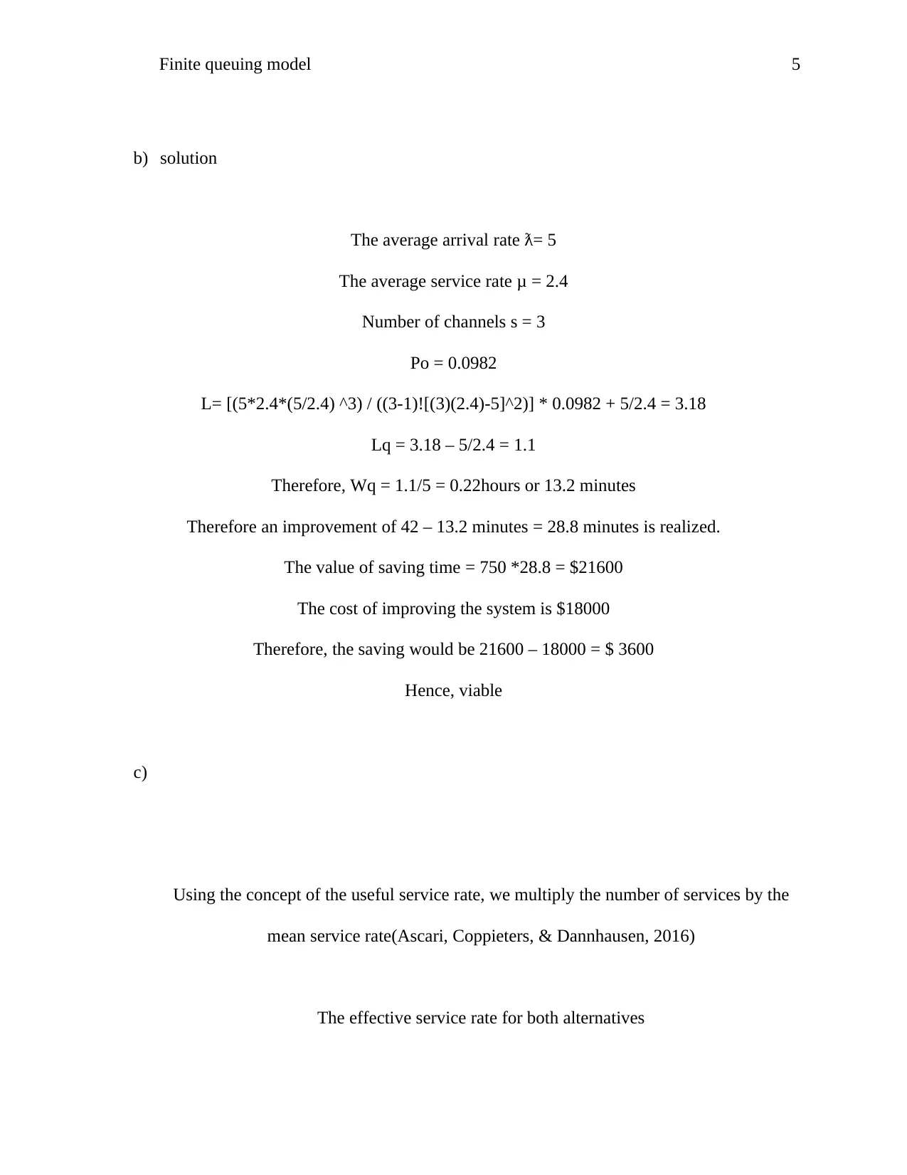
The average arrival rate ƛ= 5
The average service rate μ = 2.4
Number of channels s = 3
Po = 0.0982
L= [(5*2.4*(5/2.4) ^3) / ((3-1)![(3)(2.4)-5]^2)] * 0.0982 + 5/2.4 = 3.18
Lq = 3.18 – 5/2.4 = 1.1
Therefore, Wq = 1.1/5 = 0.22hours or 13.2 minutes
Therefore an improvement of 42 – 13.2 minutes = 28.8 minutes is realized.
The value of saving time = 750 *28.8 = $21600
The cost of improving the system is $18000
Therefore, the saving would be 21600 – 18000 = $ 3600
Hence, viable
c)
Using the concept of the useful service rate, we multiply the number of services by the
mean service rate(Ascari, Coppieters, & Dannhausen, 2016)
The effective service rate for both alternatives

Finite queuing model 6
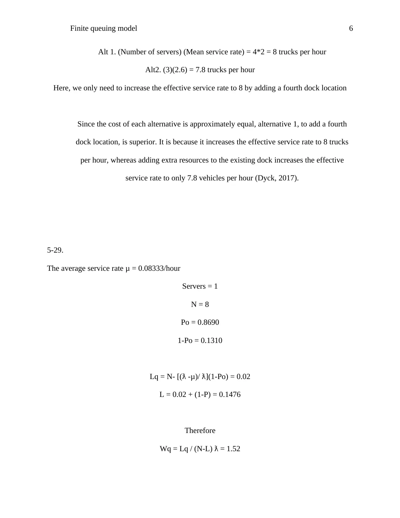
Alt 1. (Number of servers) (Mean service rate) = 4*2 = 8 trucks per hour
Alt2. (3)(2.6) = 7.8 trucks per hour
Here, we only need to increase the effective service rate to 8 by adding a fourth dock location
Since the cost of each alternative is approximately equal, alternative 1, to add a fourth
dock location, is superior. It is because it increases the effective service rate to 8 trucks
per hour, whereas adding extra resources to the existing dock increases the effective
service rate to only 7.8 vehicles per hour (Dyck, 2017).
5-29.
The average service rate μ = 0.08333/hour
Servers = 1
N = 8
Po = 0.8690
1-Po = 0.1310
Lq = N- [(ƛ -μ)/ ƛ](1-Po) = 0.02
L = 0.02 + (1-P) = 0.1476
Therefore
Wq = Lq / (N-L) ƛ = 1.52

Finite queuing model 7
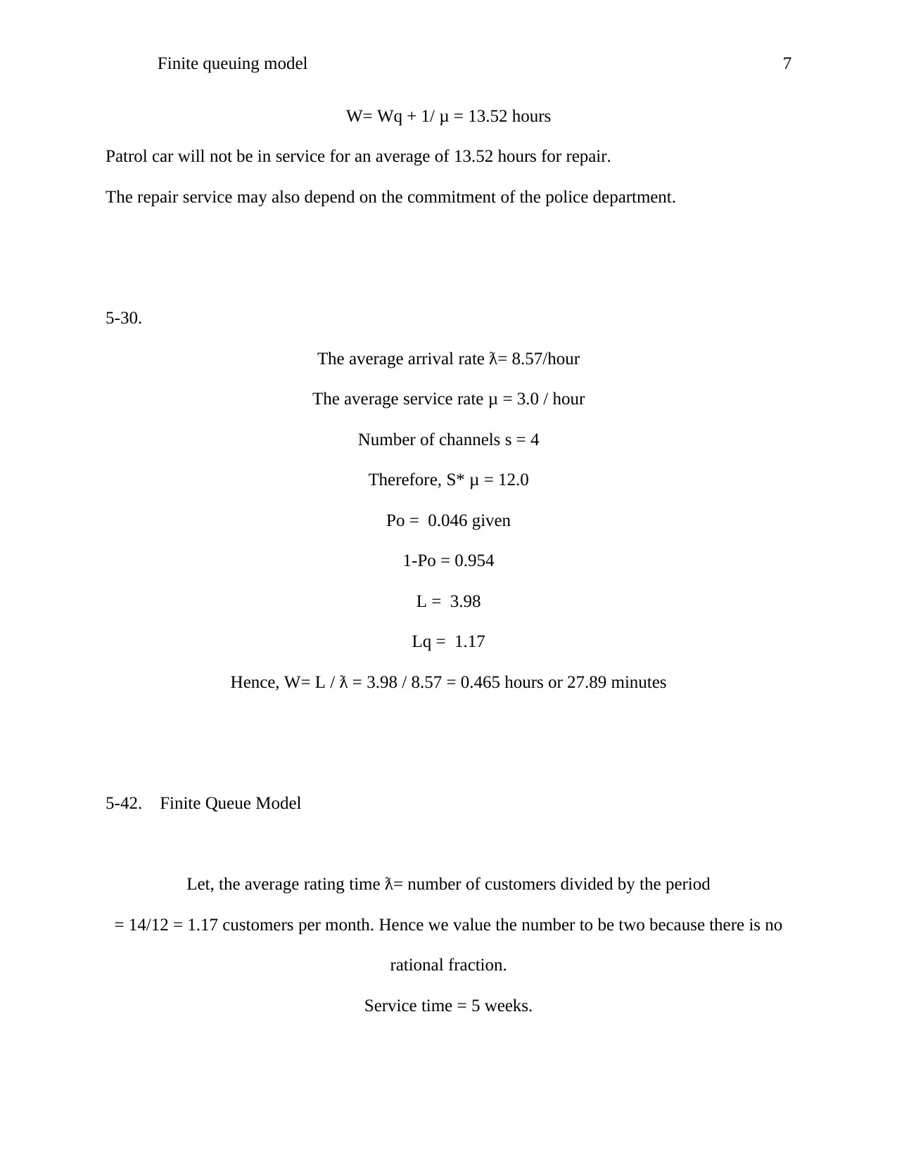
W= Wq + 1/ μ = 13.52 hours
Patrol car will not be in service for an average of 13.52 hours for repair.
The repair service may also depend on the commitment of the police department.
5-30.
The average arrival rate ƛ= 8.57/hour
The average service rate μ = 3.0 / hour
Number of channels s = 4
Therefore, S* μ = 12.0
Po = 0.046 given
1-Po = 0.954
L = 3.98
Lq = 1.17
Hence, W= L / ƛ = 3.98 / 8.57 = 0.465 hours or 27.89 minutes
5-42. Finite Queue Model
Let, the average rating time ƛ= number of customers divided by the period
= 14/12 = 1.17 customers per month. Hence we value the number to be two because there is no
rational fraction.
Service time = 5 weeks.

Finite queuing model 8
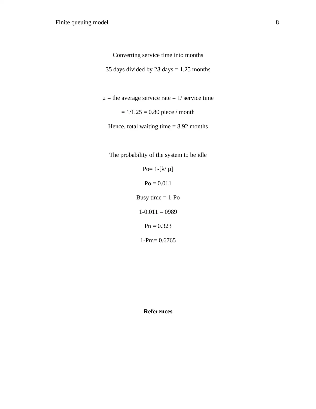
Converting service time into months
35 days divided by 28 days = 1.25 months
μ = the average service rate = 1/ service time
= 1/1.25 = 0.80 piece / month
Hence, total waiting time = 8.92 months
The probability of the system to be idle
Po= 1-[ƛ/ μ]
Po = 0.011
Busy time = 1-Po
1-0.011 = 0989
Pn = 0.323
1-Pm= 0.6765
References

Finite queuing model 9
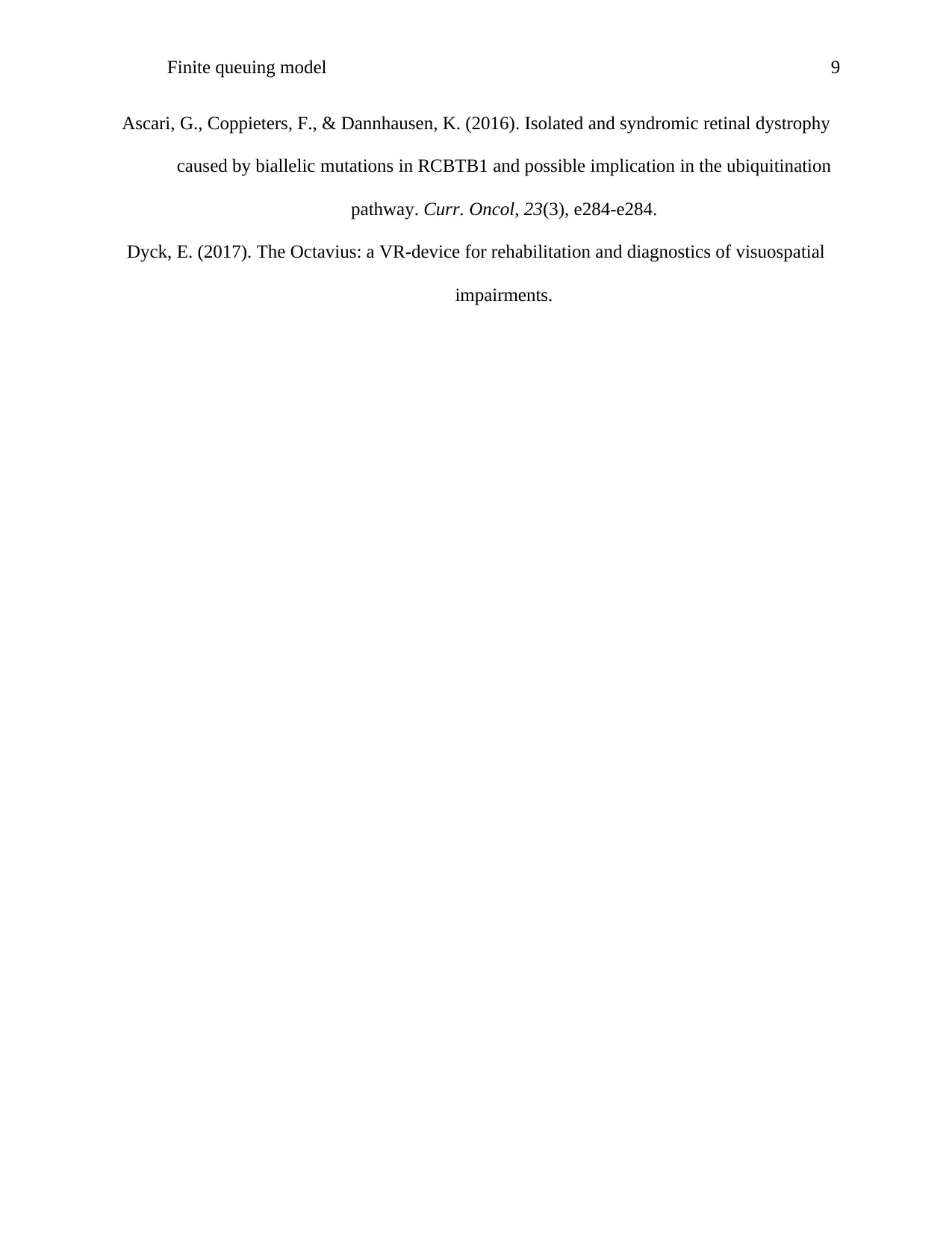
Ascari, G., Coppieters, F., & Dannhausen, K. (2016). Isolated and syndromic retinal dystrophy
caused by biallelic mutations in RCBTB1 and possible implication in the ubiquitination
pathway. Curr. Oncol, 23(3), e284-e284.
Dyck, E. (2017). The Octavius: a VR-device for rehabilitation and diagnostics of visuospatial
impairments.