Polytechnic of Namibia: BBS112S Business Statistics Assignment

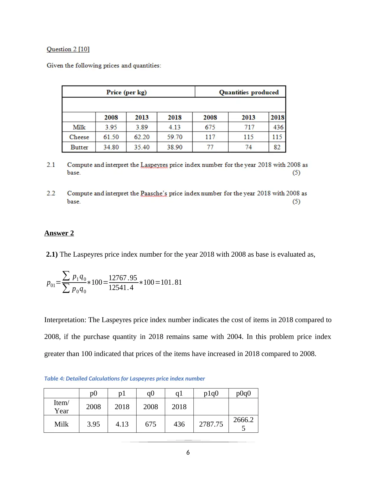
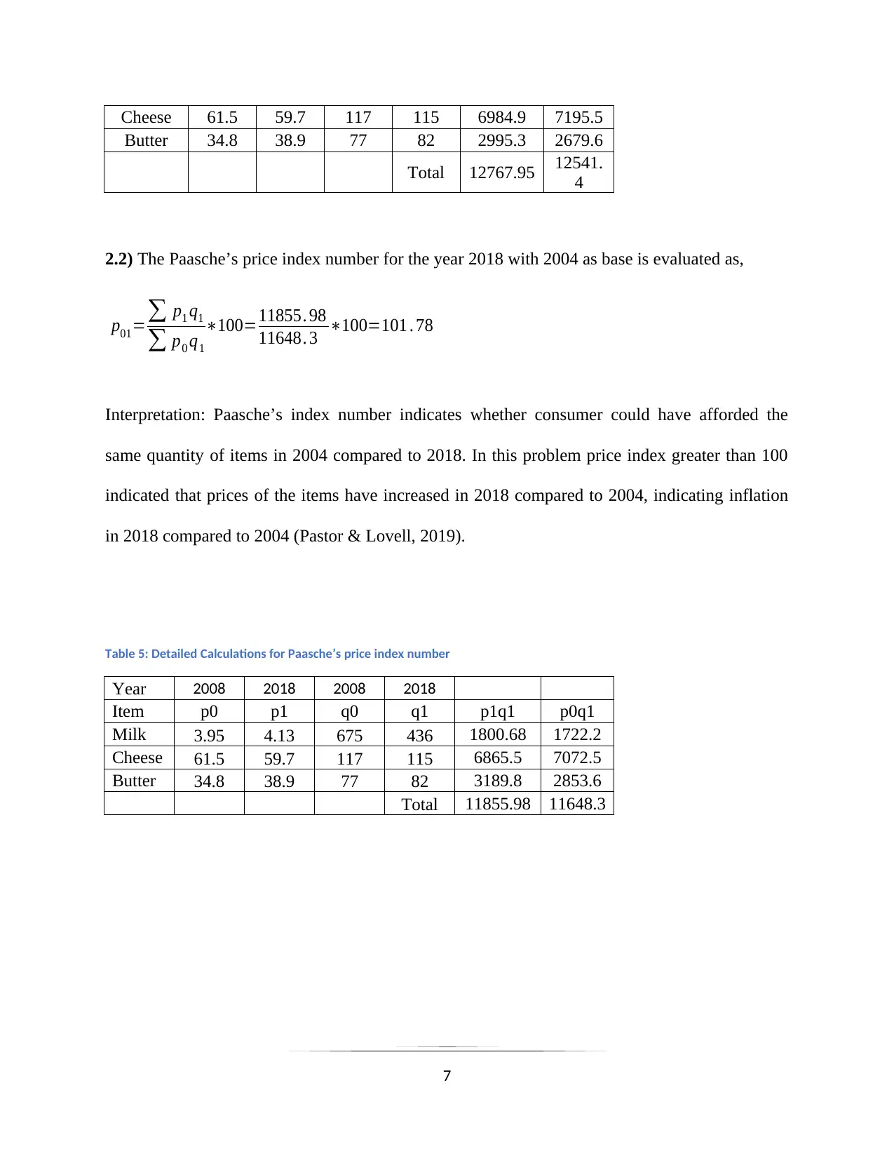
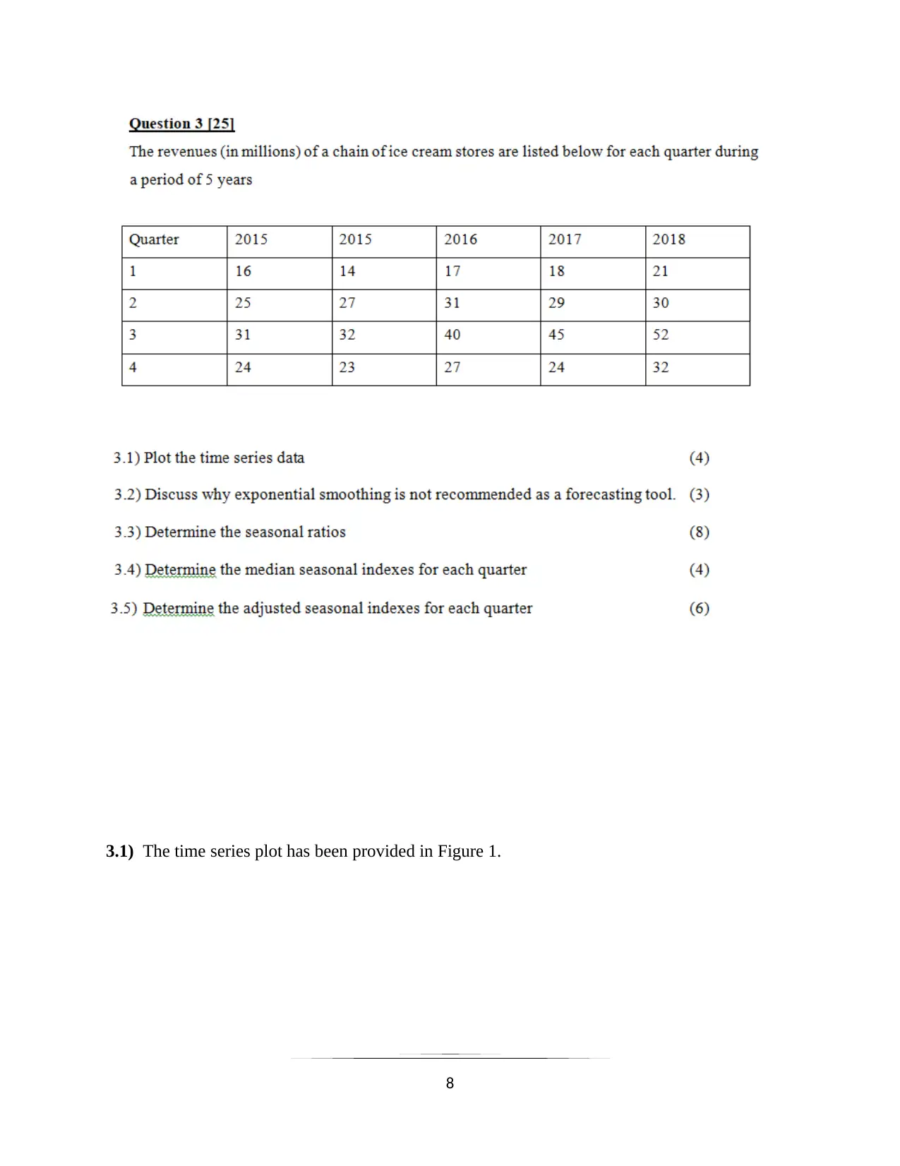
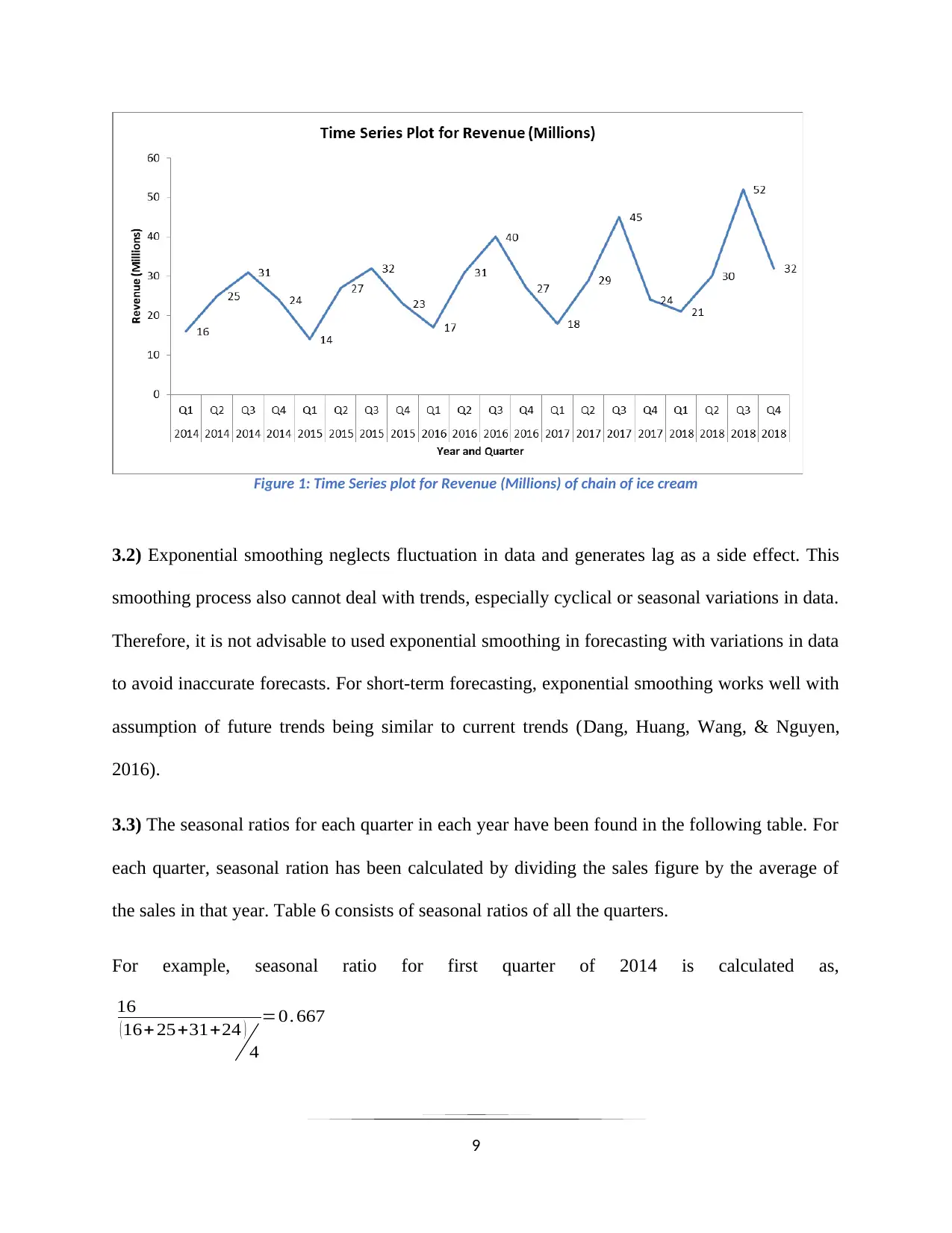
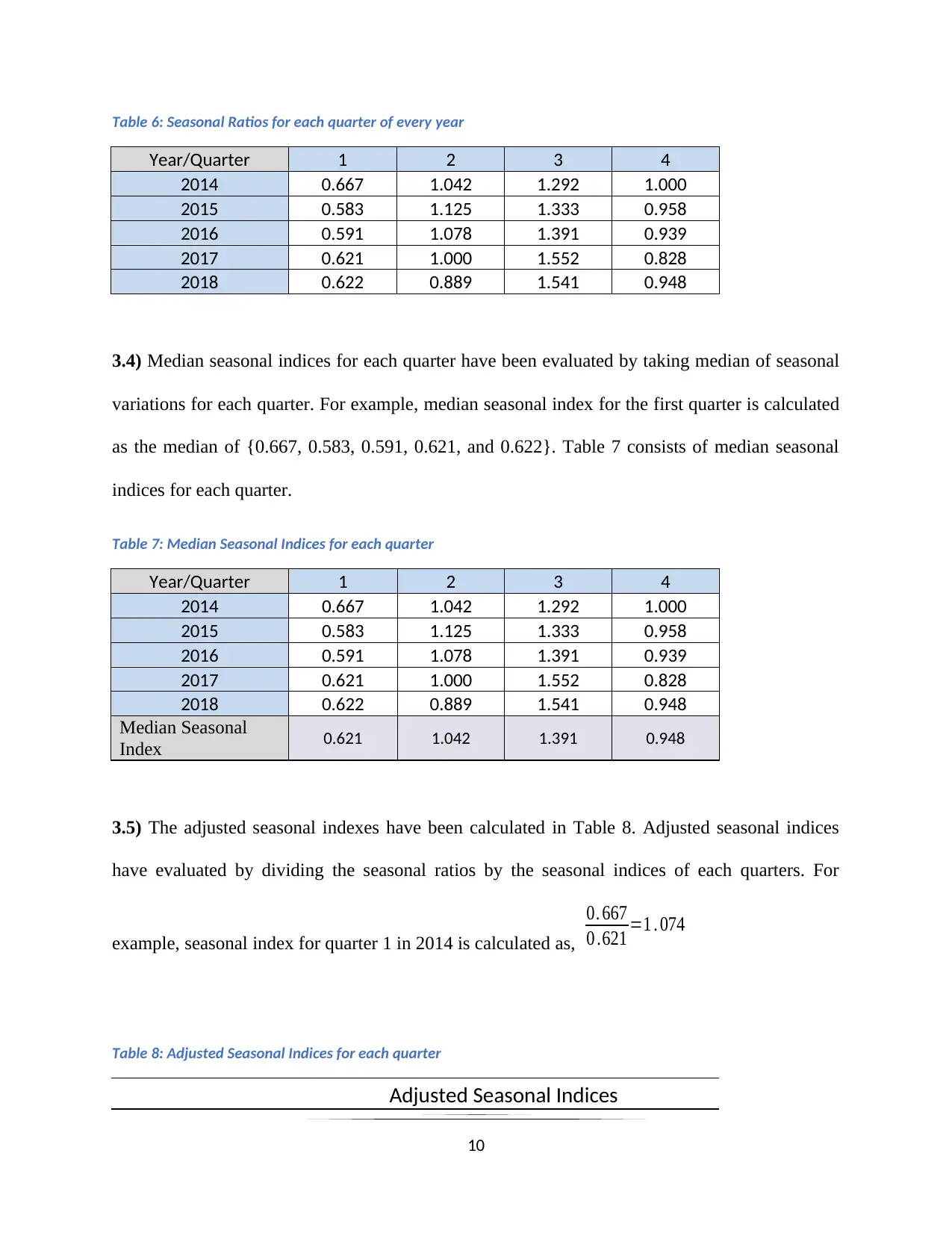
This business statistics assignment solution addresses key concepts in statistical analysis. It begins with hypothesis testing using the chi-square goodness of fit test to analyze commuter transport preferences and a one-sample F-test to evaluate the variance of cereal box weights, including confidence interval estimation. The assignment then delves into index numbers, calculating Laspeyres and Paasche price indices to assess price changes over time. Finally, the solution explores time series analysis, including time series plots, exponential smoothing, and seasonal ratio calculations to forecast ice cream sales. The solution provides detailed calculations, interpretations, and conclusions for each problem, offering a comprehensive understanding of the statistical methods applied. The references at the end of the document are based on the concepts used in the assignment.

BASICS BUSINESS STATISTICS
1

Answer
1.1.1) The expected frequencies were evaluated from the past information on percentages of
number of commuters availing transports.
The chi-square values were calculated using the formula
χ2= ( Obs−Exp ) 2
Exp for ‘N-1’
degrees of freedom. Table 1 contains the detailed calculations of Chi-square test in Excel.
Null hypothesis: There is no significant difference between the observed and expected
frequencies of residents availing the three transports.
Alternate hypothesis: There is significant difference between the observed and expected
frequencies of residents availing the three transports.
2

Significance level: Alpha = 0.05
Test statistic:
χ2= ( Obs−Exp ) 2
Exp =1 . 76+7 .56+ 12. 19=21 .51 where the p-value < 0.05.
Decision: Based on statistical evidences the null hypothesis is rejected at 5% level of
significance.
1.1.2) Conclusion: Information collected by the Mayor significantly differed from the previous
knowledge. Hence, the Mayor might conclude that choice of transport has considerably
changed in recent times.
Table 1: Chi-square test for goodness of fit for commuters with transport
3

1.2.1) The claim regarding the variance of weights of cereal boxes has been done using one
sample F-test.
Null hypothesis: The variance of cereal boxes is greater than or equal to 0.003
killograms2.
Alternate hypothesis: The variance of cereal boxes is significantly less than 0.003
killograms2.
Significance level: Alpha = 0.01
Test statistic:
χ2= ( N−1 ) s2
σ2 =121 . 20
where the χcrit
2 =1 .239
Here, χCal
2 > χCrit
2
implies that calculated statistic is in the acceptance region.
Table 2: Summary of Chi-square test statistics
Decision: Based on statistical evidences the null hypothesis failed to get rejected at 1%
level of significance.
Conclusion: Due to absence of enough statistical evidences, claim of the marketing
manager seems to be incorrect.
4

1.2.2) The 90% confidence interval was evaluated using the formula:
σ2
n−1 χ 2 ( 0. 95 , n−1 ) , σ2
n−1 χ 2 ( 0 .05 , n−1 )
.
Now,
χ2 ( 0 . 95 , n−1 ) =2. 167
χ2 ( 0 . 95 , n−1 ) =14 .067
So confidence interval is calculated as [0.0009, 0.006]
Hence, with 90% we can infer that population variance for weight of cereal boxes will be
somewhere between 0.0009 and 0.006.
Table 3: Calculation of 90% CI for population variance
Chi(0.05,7) 14.0671
Chi(0.95,7) 2.1673
Upper limit = 0.0060
Lower limit = 0.0009
90% CI
5

Answer 2
2.1) The Laspeyres price index number for the year 2018 with 2008 as base is evaluated as,
p01=∑ p1 q0
∑ p0 q0
∗100=12767 .95
12541. 4 ∗100=101. 81
Interpretation: The Laspeyres price index number indicates the cost of items in 2018 compared to
2008, if the purchase quantity in 2018 remains same with 2004. In this problem price index
greater than 100 indicated that prices of the items have increased in 2018 compared to 2008.
Table 4: Detailed Calculations for Laspeyres price index number
p0 p1 q0 q1 p1q0 p0q0
Item/
Year 2008 2018 2008 2018
Milk 3.95 4.13 675 436 2787.75 2666.2
5
6

Cheese 61.5 59.7 117 115 6984.9 7195.5
Butter 34.8 38.9 77 82 2995.3 2679.6
Total 12767.95 12541.
4
2.2) The Paasche’s price index number for the year 2018 with 2004 as base is evaluated as,
p01=∑ p1 q1
∑ p0 q1
∗100=11855. 98
11648. 3 ∗100=101 . 78
Interpretation: Paasche’s index number indicates whether consumer could have afforded the
same quantity of items in 2004 compared to 2018. In this problem price index greater than 100
indicated that prices of the items have increased in 2018 compared to 2004, indicating inflation
in 2018 compared to 2004 (Pastor & Lovell, 2019).
Table 5: Detailed Calculations for Paasche’s price index number
Year 2008 2018 2008 2018
Item p0 p1 q0 q1 p1q1 p0q1
Milk 3.95 4.13 675 436 1800.68 1722.2
Cheese 61.5 59.7 117 115 6865.5 7072.5
Butter 34.8 38.9 77 82 3189.8 2853.6
Total 11855.98 11648.3
7

3.1) The time series plot has been provided in Figure 1.
8

Figure 1: Time Series plot for Revenue (Millions) of chain of ice cream
3.2) Exponential smoothing neglects fluctuation in data and generates lag as a side effect. This
smoothing process also cannot deal with trends, especially cyclical or seasonal variations in data.
Therefore, it is not advisable to used exponential smoothing in forecasting with variations in data
to avoid inaccurate forecasts. For short-term forecasting, exponential smoothing works well with
assumption of future trends being similar to current trends (Dang, Huang, Wang, & Nguyen,
2016).
3.3) The seasonal ratios for each quarter in each year have been found in the following table. For
each quarter, seasonal ration has been calculated by dividing the sales figure by the average of
the sales in that year. Table 6 consists of seasonal ratios of all the quarters.
For example, seasonal ratio for first quarter of 2014 is calculated as,
16
( 16+ 25+31+24 )
4
=0. 667
9

Table 6: Seasonal Ratios for each quarter of every year
Year/Quarter 1 2 3 4
2014 0.667 1.042 1.292 1.000
2015 0.583 1.125 1.333 0.958
2016 0.591 1.078 1.391 0.939
2017 0.621 1.000 1.552 0.828
2018 0.622 0.889 1.541 0.948
3.4) Median seasonal indices for each quarter have been evaluated by taking median of seasonal
variations for each quarter. For example, median seasonal index for the first quarter is calculated
as the median of {0.667, 0.583, 0.591, 0.621, and 0.622}. Table 7 consists of median seasonal
indices for each quarter.
Table 7: Median Seasonal Indices for each quarter
Year/Quarter 1 2 3 4
2014 0.667 1.042 1.292 1.000
2015 0.583 1.125 1.333 0.958
2016 0.591 1.078 1.391 0.939
2017 0.621 1.000 1.552 0.828
2018 0.622 0.889 1.541 0.948
Median Seasonal
Index 0.621 1.042 1.391 0.948
3.5) The adjusted seasonal indexes have been calculated in Table 8. Adjusted seasonal indices
have evaluated by dividing the seasonal ratios by the seasonal indices of each quarters. For
example, seasonal index for quarter 1 in 2014 is calculated as,
0. 667
0 .621 =1 . 074
Table 8: Adjusted Seasonal Indices for each quarter
Adjusted Seasonal Indices
10