Statistics for Business (2018): Analysis of Household Expenditures

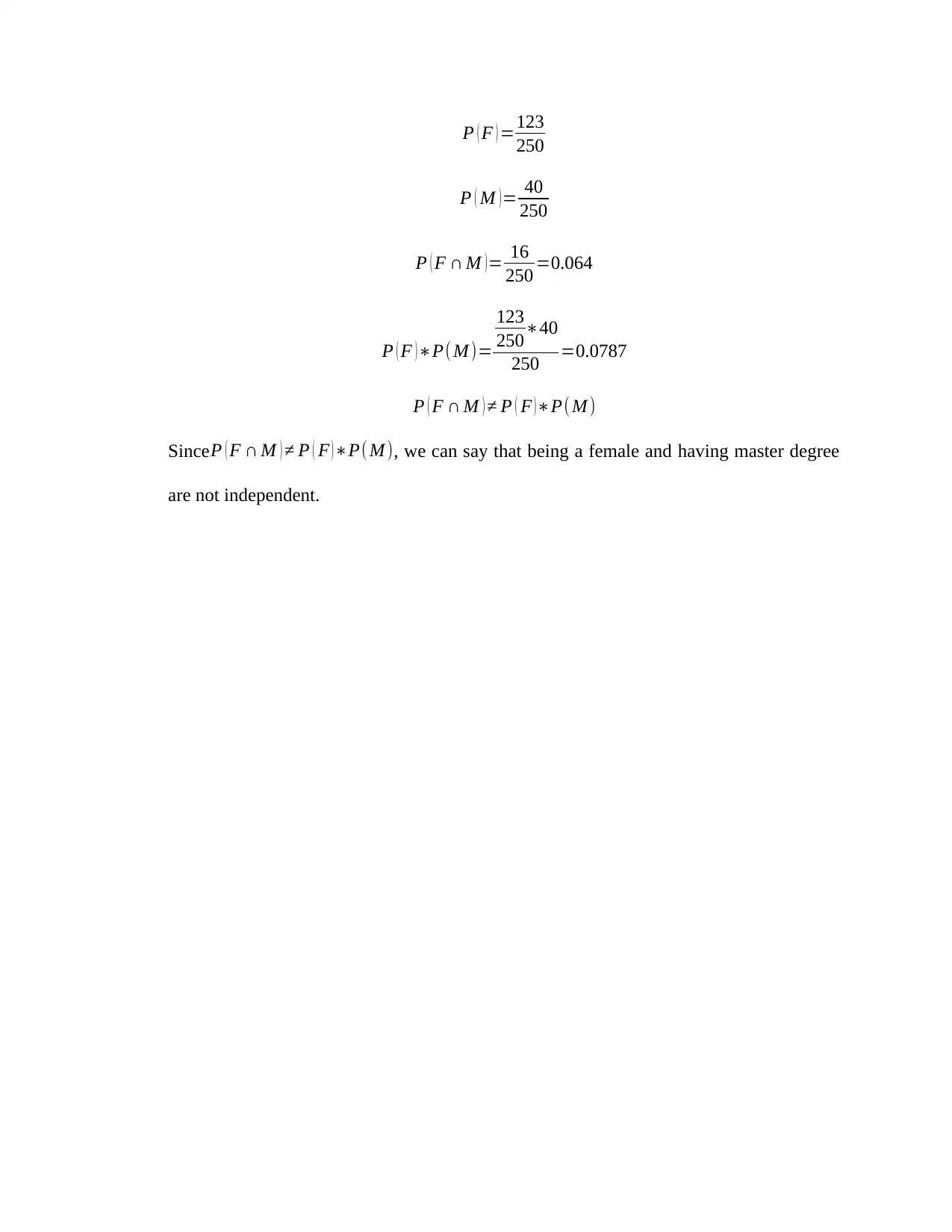
This statistics assignment analyzes household expenditure data using a random sample of 250. The solution begins with descriptive statistics for alcohol, meals, fuel, and phone expenditures, including mean, standard deviation, and a box-whisker plot to visualize the data's distribution and identify outliers. The analysis continues with the construction of a frequency distribution table for utility expenditures, followed by calculations of the percentage of households spending within specific ranges. The assignment then delves into probability calculations related to household income and ownership, including the identification of top and bottom income percentiles. A scatter plot is used to explore the correlation between after-tax income and total expenditures. Finally, a contingency table is created to examine the relationship between gender and education level, with probability calculations assessing the independence of these variables and proportions of specific demographic groups.

Statistics for Business
Student Name:
Student Number:
Date: 12th December 2018

Task 1:
A. Drawing random sample of 250
Answer
We drew a random sample of 250 samples (attached in the excel). The sampling method
used was a random sampling method. In my opinion this is not the best method especially
when one is interested in characteristics such as gender of the household head, education
level etc. this is because there is likelihood of mixing up the characteristics in the sample
and having sample with unwanted characteristics. The best sampling method would be
convenience sampling.
B. Computation of descriptive statistics and drawing a box-whisker plot of expenditure on
alcohol, meals, fuel and phone
Answer
In this section, we present the descriptive statistics for alcohol, meals, fuel and phone
expenditures.
Table 1: Descriptive Statistics
Alcohol Meals Fuel Phone
Mean 1018.58 946.57 2045.20 1342.46
Standard Error 85.40 67.35 178.89 78.74
Median 522.00 600.00 1410.00 1080.00
Mode 0.00 0.00 1200.00 1200.00
Standard Deviation 1350.24 1064.84 2828.49 1245.07
Sample Variance 1823134.91 1133887.79 8000342.36 1550192.32
Kurtosis 12.70 5.27 84.17 14.56
Skewness 2.73 2.12 7.55 3.11
Range 10949.00 6000.00 36000.00 10200.00
Minimum 0.00 0.00 0.00 0.00
Maximum 10949.00 6000.00 36000.00 10200.00
Sum 254645.00 236642.00 511300.00 335614.00
Count 250 250 250 250

Box-whisker plot
The below plot is the box-whisker plot for the four variables (alcohol, meals, fuel and
phone)
Figure 1: Whisker-box plot for expenditure on alcohol, meals, fuel and phone
C. Summary based on the descriptive and the whisker-box plot
Answer
Result showed that more expenditure went towards fuel (M = 2045.30, SD = 2828.49)
while the lowest average expenditure was on meals (M = 946.57, SD = 1064.84).
Expenditure on alcohol and phone on average was 1018.58 and 1342.46 respectively. The
whisker-box plot shows that the 4 variables had a number of outliers implying that the
four are likely to be skewed due to huge number of outliers.
The skewness values showed all the four variables were highly skewed but with the
expenditure on fuel being the most skewed (highly skewed with skewness value of 7.55)
followed by expenditure on phone with a skewness value of 3.11, meals had a skewness
of 2.12 while alcohol had a skewness value of 2.73.

Task 2:
A. Constructing the frequency distribution of expenditures on utilities
Answer
Table 2: Frequency distribution table
1 2 3 4 5 6 7 8 9 10 11
Class 0-300 300-600 600-
900
900-
1200
1200-
1500
1500-
1800
1800-
2100
2100-
2400
2400-
2700
2700-
3000
More than
3000
Frequency 16 36 46 55 28 22 16 10 8 3 10
Percent
frequency
6.4% 14.4% 18.4% 22.0% 11.2% 8.8% 6.4% 4.0% 3.2% 1.2% 4.0%
B. Percentage of households who spend on utilities
a. At the most $900 per annum
Answer
Percentage of hosueholds spending at most $ 900= ( 16 +36+ 46
250 ) ×100 %= 98
250 ×100 %=39.2 %
Thus 39.2% of the households spend at most $900 per annum
b. Between $1500 and $2700 per annum
Answer
Percentage of households spending between $ 1500∧$ 2700=( 22+1 6+10+8
250 )× 100 %= 56
250 ×100 %=
Thus 22.4% of the households spend between $1500 and $2700 per annum.
c. More than $3000 per annum
Answer
Percentage of hosueholds spending more than$ 30 00=( 10
250 )× 100 %=4 %
Thus 4% of the households spend more than $3000 per annum.
Task 3:

A. Finding the top 5% value and the bottom 5% value of the household’s annual after-tax
income
Answer
Table 3: Top 5% and bottom 5%
Top 5% value 111981
Bottom 5% value 12484.1
The two values imply that there is a large difference between the two categories hence
the data is really widely varied.
B. Let X be a random variable such that X = number of households who own a house.
(i) Is this a quantitative or a qualitative variable?
Answer
This is a qualitative variable
(ii) What would be the probability distribution when we choose (a) only 1 household
and (b) 250 households?
Answer
If only 1 household chosen then the probability distribution is;
P ( 1household chosen ) =1
2 =0.5
The condition being that we have a binary condition of either owning or not
owning a house hence the probability is assumed to equal
If 250 household chosen then the probability distribution is;
P ( 250 household chosen )=1 91
250 =0.764

In this scenario we obtain all the households who owned the house and get the
probability of owning a house based on a sample of 250 chosen.
C. Drawing a scatter plot
Answer
Figure 2: Scatter plot of ¿( Texp) against ¿( ATaxInc)
Coefficient of correlation= √0.4536=0.673 5
The coefficient of correlation is 0.6735. So looking at the graph and the coefficient of
correlation we can conclude that there is a strong positive linear relationship between
natural log of after-tax income and natural log of total expenditures.

Task 4:
A. Construct a contingency table between gender and the level of education
Answer
The table below presents the contingency table between gender and the level of
education.
Table 4: Contingency table between gender and education level
Gender of Household Head
Education level Female Male Grand Total
Primary 23 28 51
Secondary 25 26 51
Intermediate 26 23 49
Bachelors 33 26 59
Master 16 24 40
Grand Total 123 127 250
B. What is the probability that the household head is a male and has highest education level
being intermediate?
Answer
Let M be Male and I be Intermediate. So we have;
P ( M ∧I ) =P ( M ) ∗P( I )
P ( M )=127
250
P ( I ) = 49
250
P ( M∧I ) =
127
250∗49
250 =0.508∗0.196=0.0996

C. What is the probability that the household head is a female and has highest education
level being bachelors?
Answer
Let F be Feale and B be Bachelors. So we have;
P ( F ∧B ) =P ( F )∗P (B)
P ( F ) =123
250
P ( B ) = 5 9
250
P ( M∧I )=
123
250∗5 9
250 =0.492∗0.236=0.1161
D. What is the proportion of having secondary as the highest education level among the
males?
Answer
P ( Secondary )= 26
127 =0.2047=20.47 %
Thus the proportion of having secondary as the highest education level among the males
is 20.47%.
E. Do you think the events “gender of the household head is a female” and “having the
Master degree” are independent
Answer
Let Probability of female be P(F) and let probability of having master be P(M)
So we need to check whether
P ( F ∩ M ) =P ( F ) P(M )

P ( F ) =123
250
P ( M )= 40
250
P ( F ∩ M ) = 16
250 =0.064
P ( F ) ∗P( M )=
123
250∗40
250 =0.0787
P ( F ∩ M ) ≠ P ( F ) ∗P( M )
Since P ( F ∩ M ) ≠ P ( F ) ∗P( M ), we can say that being a female and having master degree
are not independent.