HI6007 Statistics: Business Data Analysis and Regression Analysis

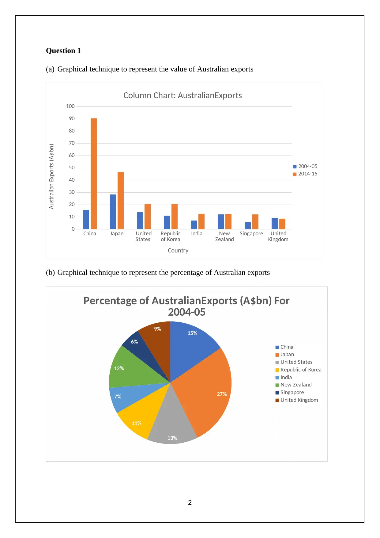
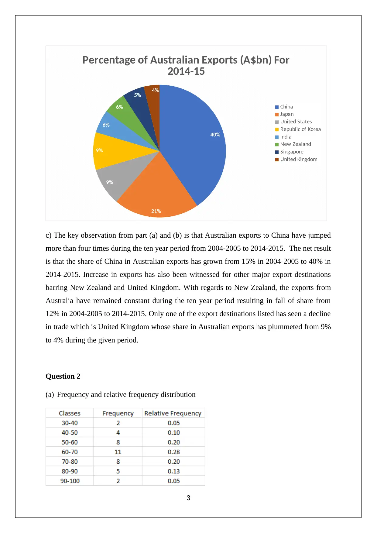
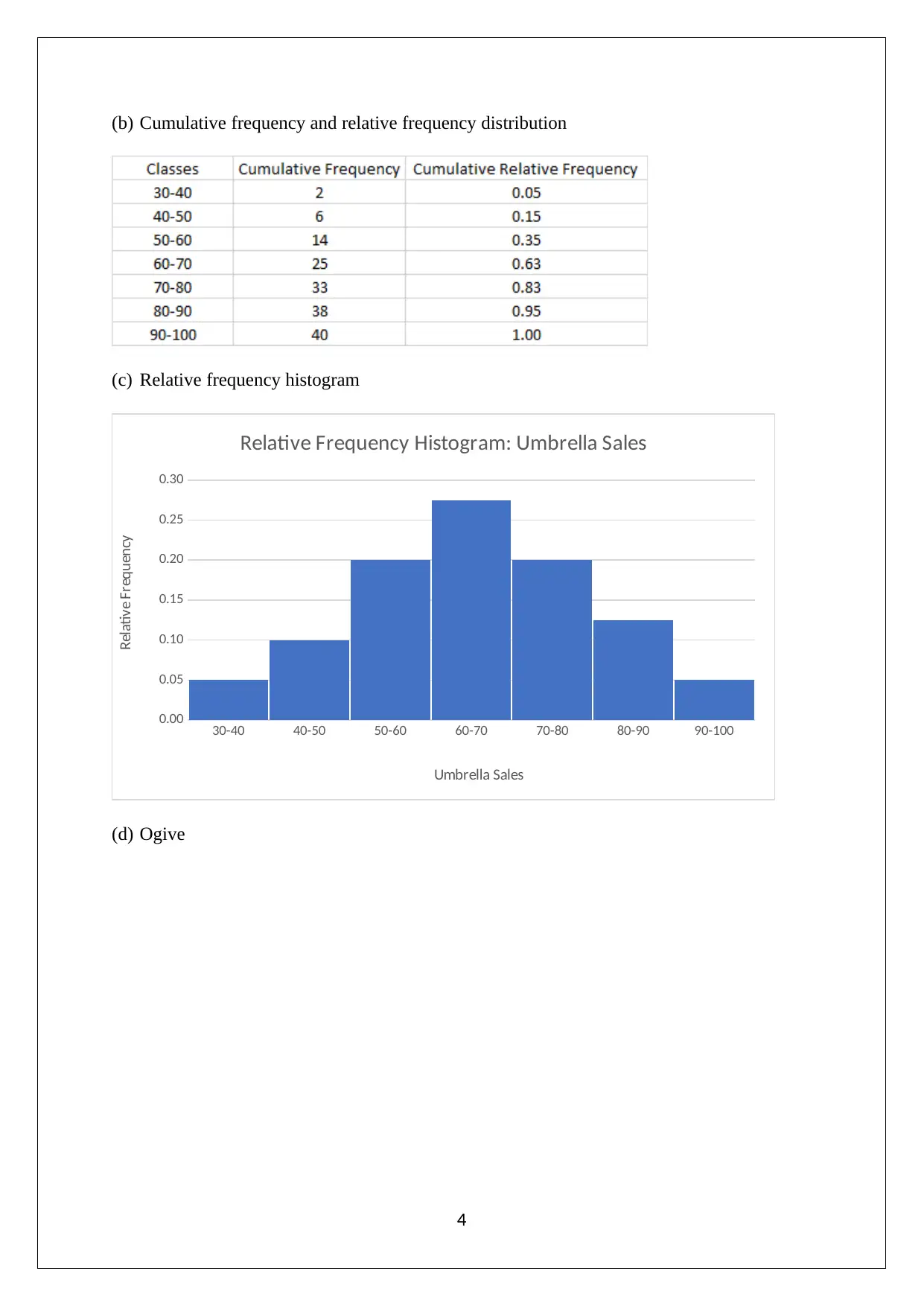
This statistics assignment analyzes business data using various statistical techniques. It begins with graphical representations of Australian exports, including column charts and percentage breakdowns, comparing data from 2004-05 and 2014-15. The assignment then delves into frequency distributions, cumulative frequencies, histograms, and ogives, using umbrella sales as an example. Time series analysis is performed on retail turnover per capita and final consumption expenditure data, with graphical representations and scatter plots illustrating relationships between variables. Further analysis includes calculating the coefficient of correlation, developing a regression equation, interpreting the slope and intercept, determining the coefficient of determination, and conducting a hypothesis test to assess the significance of the slope. The assignment concludes with an interpretation of the regression model's fit and provides relevant references.

STATISTICS FOR BUSINESS
STUDENT ID:
[Pick the date]

Question 1
(a) Graphical technique to represent the value of Australian exports
China Japan United
States Republic
of Korea India New
Zealand Singapore United
Kingdom
0
10
20
30
40
50
60
70
80
90
100
Column Chart: AustralianExports
2004-05
2014-15
Country
Australian Exports (A$bn)
(b) Graphical technique to represent the percentage of Australian exports
15%
27%
13%
11%
7%
12%
6%
9%
Percentage of AustralianExports (A$bn) For
2004-05
China
Japan
United States
Republic of Korea
India
New Zealand
Singapore
United Kingdom
2

40%
21%
9%
9%
6%
6%
5% 4%
Percentage of Australian Exports (A$bn) For
2014-15
China
Japan
United States
Republic of Korea
India
New Zealand
Singapore
United Kingdom
c) The key observation from part (a) and (b) is that Australian exports to China have jumped
more than four times during the ten year period from 2004-2005 to 2014-2015. The net result
is that the share of China in Australian exports has grown from 15% in 2004-2005 to 40% in
2014-2015. Increase in exports has also been witnessed for other major export destinations
barring New Zealand and United Kingdom. With regards to New Zealand, the exports from
Australia have remained constant during the ten year period resulting in fall of share from
12% in 2004-2005 to 2014-2015. Only one of the export destinations listed has seen a decline
in trade which is United Kingdom whose share in Australian exports has plummeted from 9%
to 4% during the given period.
Question 2
(a) Frequency and relative frequency distribution
3

(b) Cumulative frequency and relative frequency distribution
(c) Relative frequency histogram
30-40 40-50 50-60 60-70 70-80 80-90 90-100
0.00
0.05
0.10
0.15
0.20
0.25
0.30
Relative Frequency Histogram: Umbrella Sales
Umbrella Sales
Relative Frequency
(d) Ogive
4

30-40 40-50 50-60 60-70 70-80 80-90 90-100
0
5
10
15
20
25
30
35
40
45
Ogive: Umbrella Sales
Umbrella Sales
Cumulative Frequency
(e) Proportion of grade is less than 60
= 0.05 + 0.10 + 0.20 = 0.35
(f) Proportion of grade is less than 70
= 0.20 + 0.13 + 0.05 = 0.38
Question 3
(a) Time series graphical representation
5

Sep-1983
Dec-1984
Mar-1986
Jun-1987
Sep-1988
Dec-1989
Mar-1991
Jun-1992
Sep-1993
Dec-1994
Mar-1996
Jun-1997
Sep-1998
Dec-1999
Mar-2001
Jun-2002
Sep-2003
Dec-2004
Mar-2006
Jun-2007
Sep-2008
Dec-2009
Mar-2011
Jun-2012
Sep-2013
Dec-2014
Mar-2016
0.0
500.0
1000.0
1500.0
2000.0
2500.0
3000.0
3500.0
Retail turnover per capita
Time
Retail Turnover per capital ($)
Sep-1983
Jan-1985
May-1986
Sep-1987
Jan-1989
May-1990
Sep-1991
Jan-1993
May-1994
Sep-1995
Jan-1997
May-1998
Sep-1999
Jan-2001
May-2002
Sep-2003
Jan-2005
May-2006
Sep-2007
Jan-2009
May-2010
Sep-2011
Jan-2013
May-2014
Sep-2015
0
50000
100000
150000
200000
250000
FINAL CONSUMPTION EXPENDITURE
Time
Final consuption expenditure ($ million)
(b) Scatter plot to represent the relationship between variables
6

1200.0 1400.0 1600.0 1800.0 2000.0 2200.0 2400.0 2600.0 2800.0 3000.0 3200.0
0
50000
100000
150000
200000
250000
Scatter Plot
Retail turnover per capita ($)
Final Consumption Expenditure ($Million)
The retail turnover per capita has been listed on the X axis since it is the independent variable
while the final consumption is the dependent variable which is listed on the Y axis.
(c) Numerical summary
(d) Coefficient of correlation between the variables
7

The positive correlation coefficient implies that the two variables tend to show a positive
relationship with both increasing simultaneously. Further, the magnitude is quite close to 1
which implies that the underlying relationship between the two variables is very strong
(Flick,2015).
(e) Regression output
Based on the above output, the regression equation can be derived as shown below.
Regression line
Y =bo+b 1 x
Here,
Y =Final consumption expenditure ( $ million )
X =Retail turnover per capita($)
Intercept=bo=−42102.53
Slope=b 1=85.29
Hence,
Y =bo+b 1 x
Final consumption expenditure ($ million) =-42102.53+ (85.29*Retail turnover per capita($))
 The slope implies that for 1 unit increase in retain turnover per capital will increase
the final consumption expenditure by 85.29 units.
 The intercept implies that for zero retail turnover per capita, the final consumption
expenditure would be -$42102.53 million.
8

(f) Coefficient of determination
R square = 0.9755
The value indicates that 97.55% variation in final consumption expenditure would be
explained by variation in retail turnover per capita. The value is significant high and close to
1 which indicates that the model is considered to be a good fit. (Hair et. al.,2015).
(g) Hypothesis Test
Null hypothesis H0 : β=0Slope is not significant.
Alternative hypothesis Ha : β ≠ 0Slope is significant.
The slope coefficient = 85.29
The t value = 71.74
The p value = 0.00
Significance level = 0.05
It can be seen that the p value is lower than significance level and thus, null hypothesis will
be rejected and alternative will be accepted. Therefore, it can be said that slope is significant.
Thus, the variable retain turnover per capital is significant (Fehr and Grossman, 2016). The
slope implies that for 1 unit increase in retain turnover per capital will increase the final
consumption expenditure by 85.29 units.
(h) The standard error for the given regression model is 7,363.2252. The given regression
model is a good fit which can be concluded owing to the slope being significant and also
the R2 value being close to1 which would indicate high predictive power along with
significance of the underlying relationship (Eriksson and Kovalainen, 2015).
9

References
Eriksson, P. and Kovalainen, A. (2015) Quantitative methods in business research. 3rd ed.
London: Sage Publications, pp. 123-124
Fehr, F. H. and Grossman, G. (2016). An introduction to sets, probability and hypothesis
testing. 3rd ed. Ohio: Heath, pp. 145
Flick, U. (2015) Introducing research methodology: A beginner's guide to doing a research
project. 4th ed. New York: Sage Publications, pp. 167, 176
Hair, J. F., Wolfinbarger, M., Money, A. H., Samouel, P., and Page, M. J. (2015) Essentials
of business research methods. 2nd ed. New York: Routledge, pp. 199-200
10

11