Applied Statistics in Business: Data Analysis and Hypothesis Testing

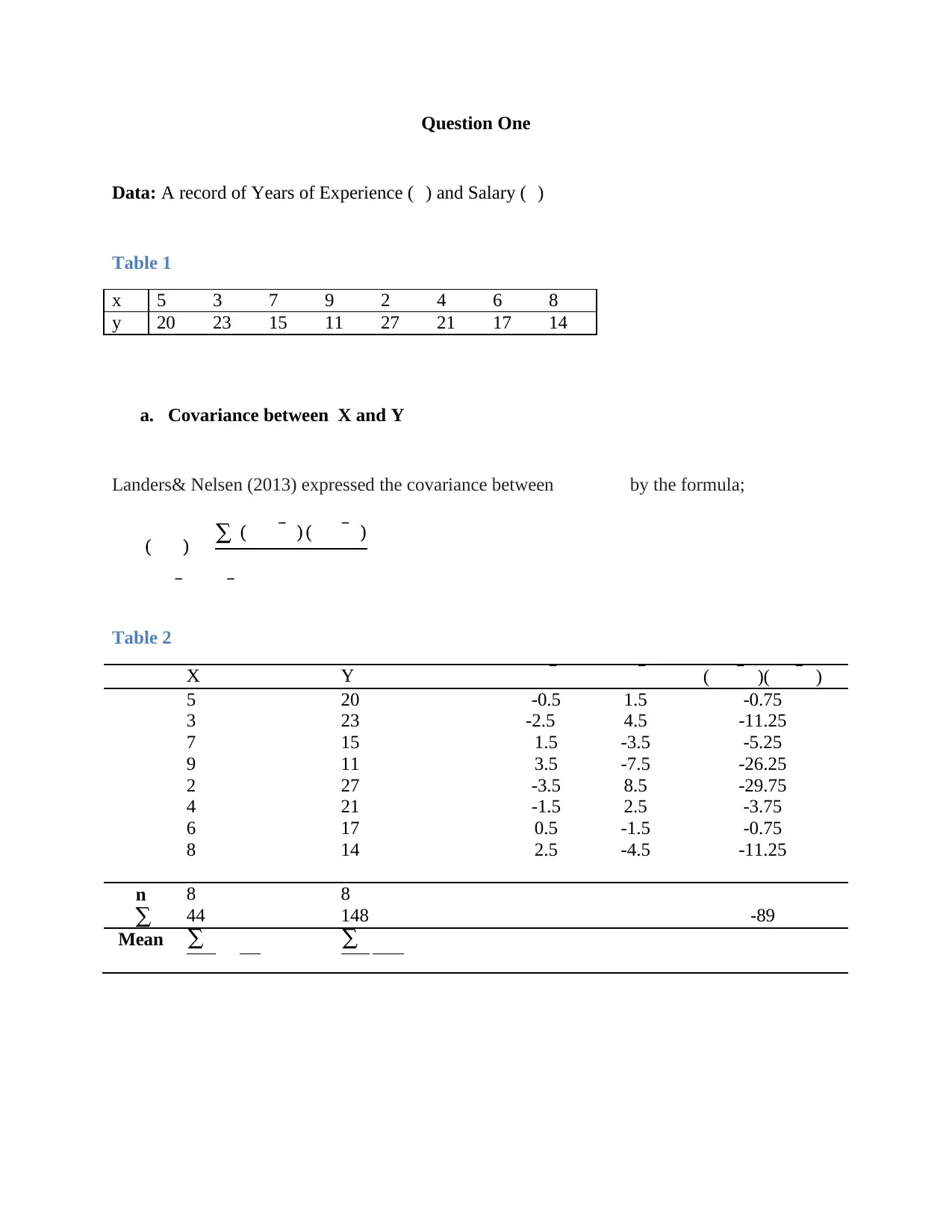
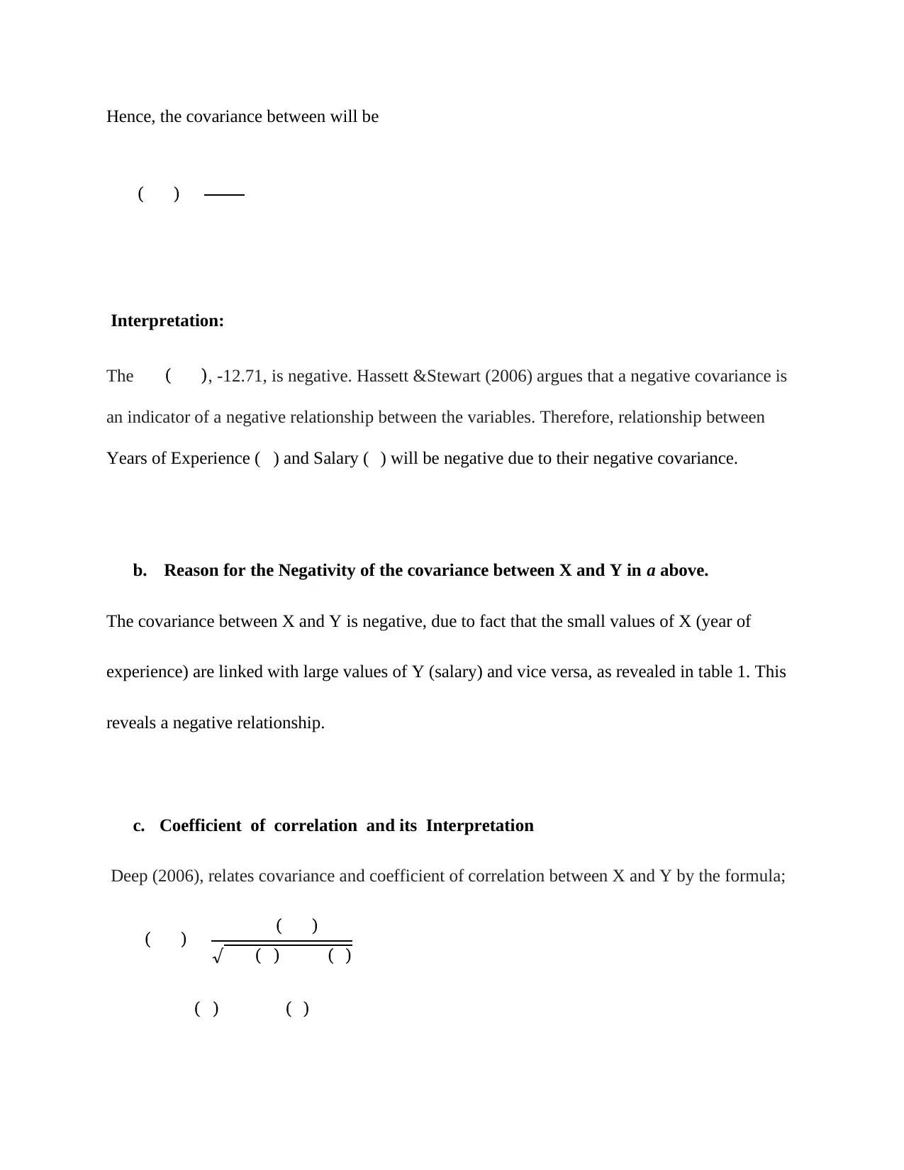
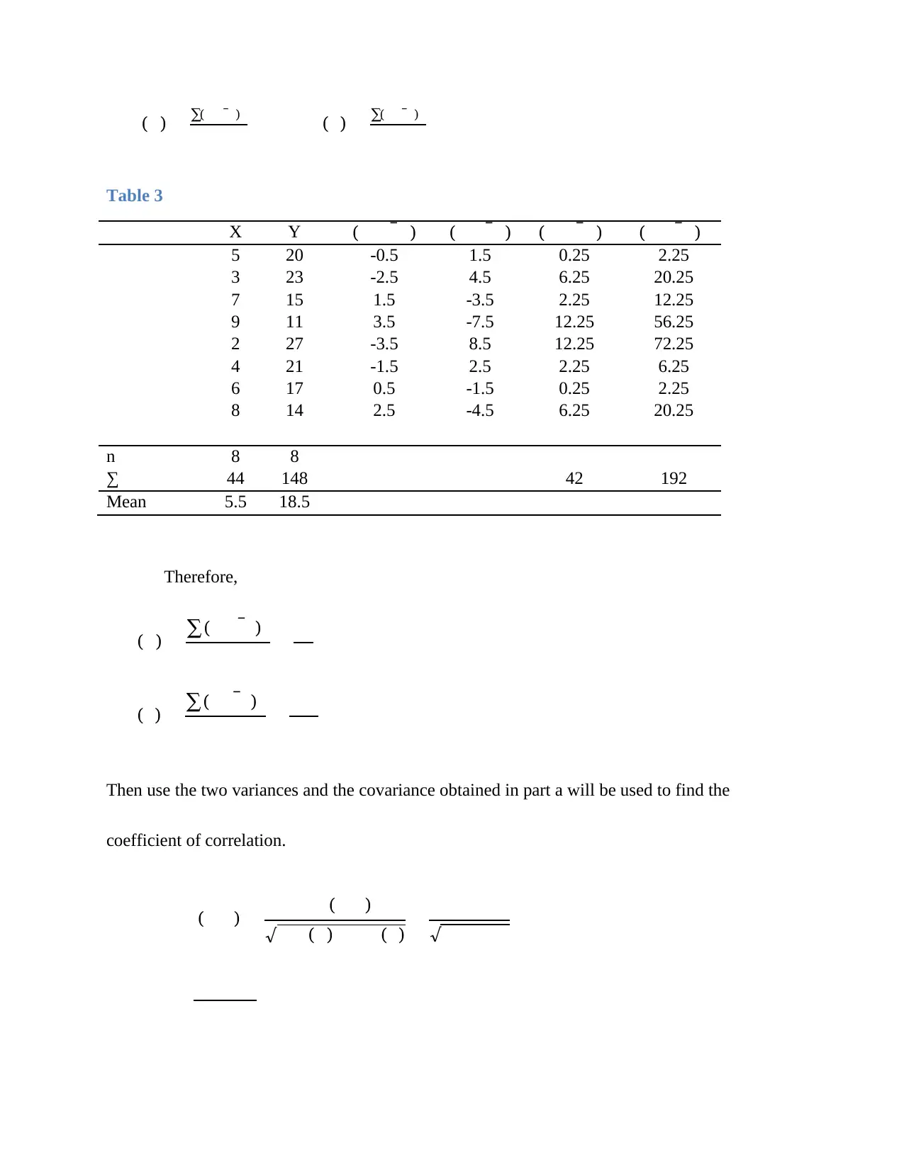
This document presents a comprehensive solution to a business statistics assignment, covering various statistical concepts and their application in business scenarios. The assignment includes problems related to covariance and correlation analysis, where the relationship between years of experience and salary is analyzed. It also delves into hypothesis testing, specifically focusing on Type II errors and the power of the test. Furthermore, the solution explores exponential distribution, calculating probabilities related to customer waiting times. The document provides detailed calculations and interpretations for each problem, offering a clear understanding of the statistical methods employed. Students can find more solved assignments and past papers on Desklib to aid in their studies.

Statistics for Business Assignment
Student’s Name
Course Code
Student’s Number
Institution Affiliation

Question One
Data: A record of Years of Experience ( ) and Salary ( )
Table 1
x 5 3 7 9 2 4 6 8
y 20 23 15 11 27 21 17 14
a. Covariance between X and Y
Landers& Nelsen (2013) expressed the covariance between by the formula;
( ) ∑ (̅ )(̅ )̅̅
Table 2
X Y̅̅ (̅ )(̅ )
5 20 -0.5 1.5 -0.75
3 23 -2.5 4.5 -11.25
7 15 1.5 -3.5 -5.25
9 11 3.5 -7.5 -26.25
2 27 -3.5 8.5 -29.75
4 21 -1.5 2.5 -3.75
6 17 0.5 -1.5 -0.75
8 14 2.5 -4.5 -11.25
n 8 8
∑ 44 148 -89
Mean ∑ ∑

Hence, the covariance between will be
( )
Interpretation:
The ( ), -12.71, is negative. Hassett &Stewart (2006) argues that a negative covariance is
an indicator of a negative relationship between the variables. Therefore, relationship between
Years of Experience ( ) and Salary ( ) will be negative due to their negative covariance.
b. Reason for the Negativity of the covariance between X and Y in a above.
The covariance between X and Y is negative, due to fact that the small values of X (year of
experience) are linked with large values of Y (salary) and vice versa, as revealed in table 1. This
reveals a negative relationship.
c. Coefficient of correlation and its Interpretation
Deep (2006), relates covariance and coefficient of correlation between X and Y by the formula;
( ) ( )
√ ( ) ( )
( ) ( )

( ) ∑(̅ ) ( ) ∑(̅ )
Table 3
X Y (̅ ) (̅ ) (̅ ) (̅ )
5 20 -0.5 1.5 0.25 2.25
3 23 -2.5 4.5 6.25 20.25
7 15 1.5 -3.5 2.25 12.25
9 11 3.5 -7.5 12.25 56.25
2 27 -3.5 8.5 12.25 72.25
4 21 -1.5 2.5 2.25 6.25
6 17 0.5 -1.5 0.25 2.25
8 14 2.5 -4.5 6.25 20.25
n 8 8
∑ 44 148 42 192
Mean 5.5 18.5
Therefore,
( ) ∑(̅ )
( ) ∑(̅ )
Then use the two variances and the covariance obtained in part a will be used to find the
coefficient of correlation.
( ) ( )
√ ( ) ( ) √

Therefore, the correlation coefficient(X, Y) is -0.9911, which is negative and near to -1. This
shows that the correlation between X (years of experience) and Y (salary) is high and negative.
Just like the covariance, it reveals that X and Y are highly negatively related.
d. Reason for the negative correlation coefficient.
The correlation coefficient between X and Y is negative since the covariance which influences
the sign of correlation level is negative.
Question Two
Data: mean of an exponential distribution is 3 minute
According to Ross (2014), the following are the features of exponential distribution:
 Probability density function (pdf) of exponential distribution
( )
 Expectation of T is given by
 Cumulative probability function (Cdf) is given by
( ) ∫ ( )

a. The value of a parameter for the exponential distribution
( )
b. Customers’ proportion, who holds for more than 1.5 minutes.
This will be computed by integrating the pdf of exponential distribution between 1.5 and
infinity.
∫
{
( )
c. Waiting time at which 10% of the customer will continue to hold.
This will be computed from the probability that , which can computed from the Cdf of the
exponential distribution as shown below.

( ) ∫( )
Therefore,
( )
d. Probability a randomly selected customer is placed on hold for 3 to 6 minutes.
This will be given by ( ) ( ) , which can be computed using the Cdf Formula
( ) ∫( )
( )
( )
Hence, ( ) ( )

Question Three
Data: H0: = 950 hours vs. H1: 950 hours, ( )
( )
a. Calculation of (probability of a Type II error) when = 1000 and = 0.10.
First, the critical value of sample mean will be computed. Goos & Meintrup (2016), express the
critical value of sample mean as;
√
√ √
Thus critical mean will be
Therefore,
( . This is computed as follows using z-scores and it’s
probabilities from tables
( ) ( | √ )
( ) ( )

( ) ( )
Thus,
b. Computation of power of the test when = 1000 and = 0.10.
The power of the test is computed by the formula
c. Interpretation of the power of the test
, is the probability of correctly rejecting the null hypothesis that , when
the population mean is indeed 1000
d. Effects of increasing the sample size.
To illustrate this, another shall be computed using a different sample of size 49. Formulae in
Part a above will be utilized
√
√ √

(
This given by
( ) ( | √ )
( ) ( )
( ) ( )
Thus, , which is less than initial . This reveals that when sample
size is increase, the probability of a Type II error( ) will decrease. On the other hands, the
power of test will increase as it depends on the value of , a smaller leads to a bigger power
of test.

Question Four
Data: A record of Production Filling Operations
( ) ( ) ,
, ( ̅ )
Hypotheses to be tested at 5% significance level
The hypotheses will be based on -score as the standard deviation are known. Francis (2004)
expresses -score by the formula;̅
√
√
Thus, -score computed is 1.6
The critical value of z will then be determined from the z-tables at 5% significance level, to help
in decision in making. Since,the above test is left-tailed, the critical will be -1.645, which is
absolutely greater than , 1.6.

Interpretation:
The computed is less than the critical value of therefore, null hypothesis will not be rejected
(Ruppert, 2014). This shows that the population mean is not less than 47 at 5% significance
level.