Monash University Business Statistics 1: Data Analysis Assignment

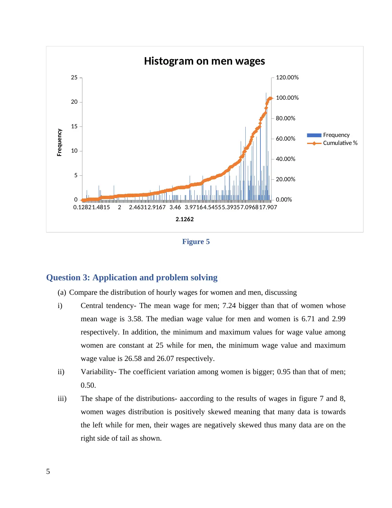
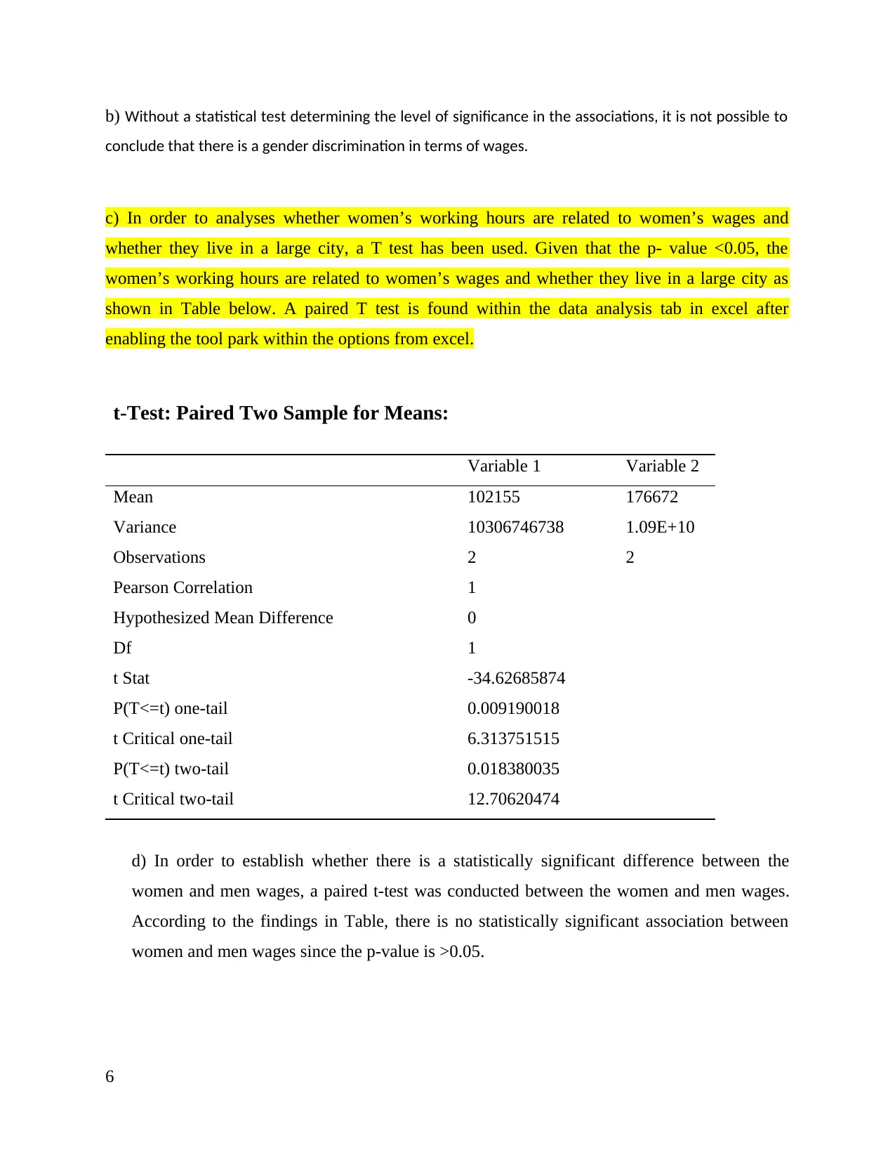
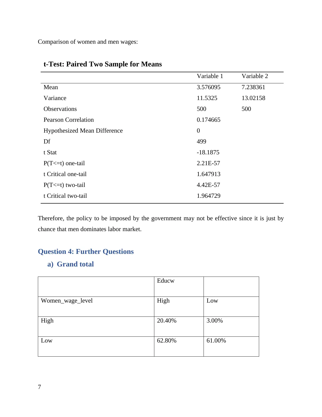
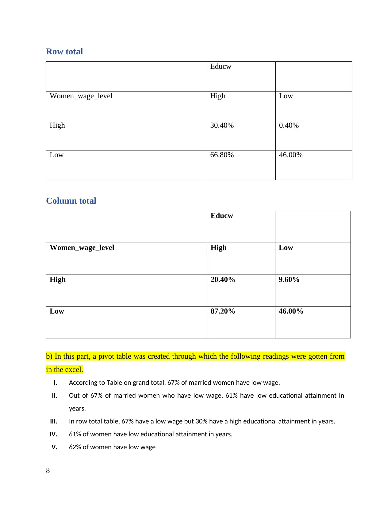
This assignment analyzes a dataset related to women's wages and working hours, employing various statistical techniques. The solution begins by classifying variables and identifying the data type, followed by calculating proportions and performing preliminary analyses to compare hourly wages based on different criteria such as the presence of preschool children, age, and working hours. Descriptive statistics, including mean, median, standard deviation, and interquartile range, are calculated and compared for wages. The assignment further explores the distribution of hourly wages for men and women, discussing central tendency, variability, and the shape of the distributions. T-tests are used to assess the relationship between women's working hours, wages, and location, as well as to determine if there is a statistically significant difference between women's and men's wages. Pivot tables and chi-square tests are also employed to analyze the relationship between educational attainment, wage levels, and working hours. Finally, probabilities are calculated based on the dataset, providing a comprehensive statistical analysis of the provided data.

PART B
Question 1: Understanding your data
(a) Qualitative variable: Live in a large city is a nominal variable because it gives
categories which is either yes or no.
Quantitative variable: Wife’s hours of work in 1975 which is continuous variable
because it measured through counting.
(b) The data is cross sectional because it is a one point of time collection of data in 1975. In a
cross-sectional study, a snap point of information is collected without considering what
happens after data collection.
(c) The proportion of working women having children under the age of 6 is given by
53/500*100% which approximately 9%.
Question 2: Preliminary analysis
(a) Compare the hourly wage, on average, for women who:
i. Have preschool children (less than 6 years old) vs. no preschool child/children
920.9; 41%
1350.6; 59%
Have preschool children (less than 6 years old) No preschool child/children
Figure 1
1

The hourly wage, on average, for women who have preschool children (less than 6 years old) is
higher; 59% compared to those without preschool child/children as shown in the figure above.
ii) Are less than 45 years old vs. not less than 45 years old.
Are less than 45 years old Not less than 45 years old
1240
1260
1280
1300
1320
1340
1360
1277.8
1339.3
Hourly wage among women
Figure 2
The mean average for women who are not less than 45 years old are higher; 1339.3 compared to
women who are less than 45 years old; 1277.8 as shown in the graph above.
iii) Have long working hours (more than 1200 hours in 1975) vs. no long working hours
The mean average for women who have long working hours (more than 1200 hours in 1975)
1345 compared to 988 among women with no long working hours as shown in the graph above.
2

Have long working hours (more than 1200 hours in 1975) No long working hours
1345
988
Hourly wage among women
Figure 3
In question 2b, the excel functions such as average, median, standard deviation etc have been
used to pull out answers as shown in the Table below.
2 (b)
Wage ($) Wife Husband
Mean 3.58 7.24
Median 2.99 6.71
Standard Deviation 3.39 3.60
First Quartile 1.64 4.83
Third Quartile 4.61 8.86
Interquartile Range 2.97 4.04
Minimum 0.00 0.51
Maximum 25.00 26.58
Range 25.00 26.07
Coefficient of Variation 0.95 0.50
Count 500.00 500.00
c)
3

0.51283.1056 4.183 4.87875.49676.22786.74167.30618.17769.0543 10.05 12.789
0
5
10
15
20
25
0.00%
20.00%
40.00%
60.00%
80.00%
100.00%
120.00%
Histogram for Women wages
Frequency
Cumulative %
4.2206
Frequency
Figure 4
4

0.12821.4815 2 2.46312.9167 3.46 3.97164.54555.39357.096817.907
0
5
10
15
20
25
0.00%
20.00%
40.00%
60.00%
80.00%
100.00%
120.00%
Histogram on men wages
Frequency
Cumulative %
2.1262
Frequency
Figure 5
Question 3: Application and problem solving
(a) Compare the distribution of hourly wages for women and men, discussing
i) Central tendency- The mean wage for men; 7.24 bigger than that of women whose
mean wage is 3.58. The median wage value for men and women is 6.71 and 2.99
respectively. In addition, the minimum and maximum values for wage value among
women are constant at 25 while for men, the minimum wage value and maximum
wage value is 26.58 and 26.07 respectively.
ii) Variability- The coefficient variation among women is bigger; 0.95 than that of men;
0.50.
iii) The shape of the distributions- aaccording to the results of wages in figure 7 and 8,
women wages distribution is positively skewed meaning that many data is towards
the left while for men, their wages are negatively skewed thus many data are on the
right side of tail as shown.
5

b) Without a statistical test determining the level of significance in the associations, it is not possible to
conclude that there is a gender discrimination in terms of wages.
c) In order to analyses whether women’s working hours are related to women’s wages and
whether they live in a large city, a T test has been used. Given that the p- value <0.05, the
women’s working hours are related to women’s wages and whether they live in a large city as
shown in Table below. A paired T test is found within the data analysis tab in excel after
enabling the tool park within the options from excel.
t-Test: Paired Two Sample for Means:
Variable 1 Variable 2
Mean 102155 176672
Variance 10306746738 1.09E+10
Observations 2 2
Pearson Correlation 1
Hypothesized Mean Difference 0
Df 1
t Stat -34.62685874
P(T<=t) one-tail 0.009190018
t Critical one-tail 6.313751515
P(T<=t) two-tail 0.018380035
t Critical two-tail 12.70620474
d) In order to establish whether there is a statistically significant difference between the
women and men wages, a paired t-test was conducted between the women and men wages.
According to the findings in Table, there is no statistically significant association between
women and men wages since the p-value is >0.05.
6

Comparison of women and men wages:
t-Test: Paired Two Sample for Means
Variable 1 Variable 2
Mean 3.576095 7.238361
Variance 11.5325 13.02158
Observations 500 500
Pearson Correlation 0.174665
Hypothesized Mean Difference 0
Df 499
t Stat -18.1875
P(T<=t) one-tail 2.21E-57
t Critical one-tail 1.647913
P(T<=t) two-tail 4.42E-57
t Critical two-tail 1.964729
Therefore, the policy to be imposed by the government may not be effective since it is just by
chance that men dominates labor market.
Question 4: Further Questions
a) Grand total
Educw
Women_wage_level High Low
High 20.40% 3.00%
Low 62.80% 61.00%
7

Row total
Educw
Women_wage_level High Low
High 30.40% 0.40%
Low 66.80% 46.00%
Column total
Educw
Women_wage_level High Low
High 20.40% 9.60%
Low 87.20% 46.00%
b) In this part, a pivot table was created through which the following readings were gotten from
in the excel.
I. According to Table on grand total, 67% of married women have low wage.
II. Out of 67% of married women who have low wage, 61% have low educational attainment in
years.
III. In row total table, 67% have a low wage but 30% have a high educational attainment in years.
IV. 61% of women have low educational attainment in years.
V. 62% of women have low wage
8

b) In this section, majority of the participants; 60.4% who do not work also do not live in the city.
However, 42.6% of those who live in the city had working hours (more than 1200 hours in 1975).
Live in city
yes no
Have long working hours (more than 1200 hours in 1975) 42.60% 57.40%
No long working hours 39.60% 60.40%
Chi-square test reveals p value <0.05 hence the women’s work hours relates to the area where
they live
In d, probabilities have been calculated based on the number of events occurring out of the total
events expressed as a percentage.
d) i) 4.6%
ii) 34.78%
iii) 34.8%
9