Statistical Analysis of ABZ Corporation Sales and Customer Data

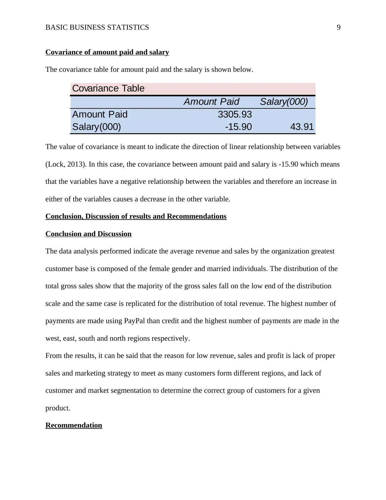
This report provides a comprehensive statistical analysis of sales and customer data from ABZ Corporation, a global company dealing with DVDs, CDs, and books. The analysis utilizes descriptive statistics, including measures of location and dispersion, to understand variables such as age, salary, and revenue. Categorical data, such as gender, customer type, and marital status, are analyzed using frequency tables and visualizations like bar and pie charts. Numeric variables, including total gross sales and revenue, are examined using frequency tables and histograms to identify distribution patterns. Pivot tables are employed to analyze relationships between region, payment methods, and sales sources. Covariance is used to assess the relationship between amount paid and salary. The report concludes with key findings, such as the importance of customer segmentation and marketing strategies, and provides recommendations to improve sales, revenue, and overall profit by targeting the right markets and optimizing resource utilization. The report is based on data from a 400-day trading period and includes a detailed description of variables, data types, and measurement scales.

Running head: BASIC BUSINESS STATISTICS 1
Basic Business Statistics
Student Name
Professor’s Name
University Name
Date

BASIC BUSINESS STATISTICS 2
Basic Business Statistics
Introduction
ABZ is a global corporation that deals with the sales of different categories of products including
DVD, CD, and books which include classical, novel, politics and bestsellers. The organization is
faced with the challenge of increasing sales, revenue and profit and thus conducts a survey and
collects data for customer demographics and sales to identify the reasons behind the problem.
The objective of this paper is to conduct statistical analysis on the data collected by the
organization with an aim of providing the best recommendations that would lead to improvement
of the sales, revenue and profit. To achieve the objective, the data is analyzed using descriptive
numerical measures and visualization graphs to draw meaningful conclusions for easy decision
making.
Description of Variables, Data Types and Measurement Scales
The table is a summary for the variables in customer attribute data, their types and levels of
measurement.
Dataset 1- Customer Attributes
Variable Type Level of Measurement Description
Customer_Id Discrete Numeric Nominal Unique ID of each customer
Gender Coded Categorical Nominal 1. Male and 2. Female
Marial Status Coded Categorical Nominal 1. Married and 2. Single
Age Continous Numeric Ratio The age of the customer
Type of Customer Coded Categorical Nominal 1. Regional and 2. Promotional
Region Coded Categorical Nominal 1. East, 2. West, 3. North and 4. South
Payment Coded Categorical Nominal 1. Paypal and 2. Credit
Source Coded Categorical Nominal 1.Web and 2. Email
Amount Paid Continous Numeric Ratio The amount paid by customer for product
Product Coded Categorical Nominal 1. DVD, 2. CD, 3. Novel, 4. Classical, 5. Politics, and 6 Best seller
Salary Continous Numeric Ratio The salary of the customer

BASIC BUSINESS STATISTICS 3
The following table describes the variables in sales data, their type and levels of measurement.
Dataset 2-Sales
Variable Type Level of Measurement Description
Days Discrete Numeric Interval Days of Transaction
Opening Gross Sales Continous Numeric Ratio Opening Gross Sales
Total Gross Sales Continous Numeric Ratio Total Gross Sales for the days
Price over earning ratio Continous Numeric Ratio Price over earning ratio
Gross profit margin Continous Numeric Ratio Gross profit margin in percentage
Revenue Continous Numeric Ratio Revenue
Descriptive Statistics for numeric variables
Descriptive statistics for numeric variables include measures of location and measures of
variation. The are summarized in the table below.
Measures of Location
Age Amount Paid Salary Opening Gorss Sales Total Gross Sales Price/Earning Ratio Gross Profit Margin Revenue
Sample average 43.08 39.79 47.47 27.51 90.47 23.57 26.32 286.46
Median 42.00 20.50 47.50 19.08 72.40 20.60 22.90 269.00
25th Percentile 32.00 17.70 44.00 12.97 39.35 8.80 9.70 252.25
75th Percentile 50.00 23.27 52.00 32.06 107.08 35.80 36.40 298.00
Measures of Variation
Variance 152.33 3314.22 44.02 697.79 4606.08 262.59 317.54 3552.81
Standard Deviation 12.34 57.57 6.63 26.42 67.87 16.20 17.82 59.61
Minimum 20.00 15.08 26.00 0.07 29.14 3.60 3.60 229.00
Maximum 78.00 246.67 65.00 169.19 381.01 68.20 74.20 539.00
Range 58.00 231.59 39.00 169.12 351.87 64.60 70.60 310.00
IQR 18 5.57 8 19.09 67.72 27.00 26.70 45.75
Descriptive Statistics for Numeric Variables
From the table above, the numeric variables are shown as columns and include age, amount paid,
salary, opening gross sales, total gross sales, price/earning ratio, gross profit margin and revenue.
The measures of location determined are the sample average, the median, 25th percentile and 75th
percentile. Sample average and mean indicate the approximate center value in the distribution of
each variable if either of the measures is chosen, the 25th and 75th percentile show that 25% and
7% of the values in a given variable distribution falls below that value. On the other hand, the
measures of dispersion or variation determined variance, standard deviation, range and
interquartile range. The range is the difference between maximum and minimum while

BASIC BUSINESS STATISTICS 4
interquartile range is the difference between the 25th percentile (1st quartile) and 75th percentile
(3rd quartile). The variable with higher values of the measures of dispersion has the highest level
of spread/dispersion.
Discussion of whether we can determine Numeric measures for Nominal and Ordinal
Categorical variables
It is not possible to determine the numeric measures of location and variation for ordinal and
categorical variables. Nominal variables are applied in the labeling of variables and have no
quantitative or numerical significance and hence not possible to determine descriptive statistics
of location and variation for them. On the hand, ordinal variables are almost similar to nominal
variables except the labels have some rank or order. The numerical measures for these types of
variables can only be expressed either as frequencies, proportions or percentages.
Data summarizing
Frequency tables and corresponding graphs for two different categorical variables
The three categorical variables selected are gender, customer type and marital status. Bar chart
and pie chart have been used as the recommended charts for visualization respectively.
Gender and Customer type
The frequency table for gender is illustrated below.
Gender Count of Type of Customer
1 28
2 372
Grand Total 400
Since code 1 represents male and code 2 represent female for gender and 1 is regular and 2
promotional for customer type, it means that the sample data had a total of 372 females who
were regular customers and 28 male individuals who were promotional. The above frequency
table can be visualized using the bar chart below.

BASIC BUSINESS STATISTICS 5
Marital Status and customer type
The frequency table for the categorical variables customer type and marital status is illustrated
below.
Marital Status Count of Type of Customer
1 336
2 64
Grand Total 400
The above frequency table above can be visualized using the pie chart below.

BASIC BUSINESS STATISTICS 6
Code 1 represents married while code 2 represents single for gender while 1 represents regular
and 2 promotional for customer type. From the numerical summary above, the sample has 336
married individuals who are regular customers and 64 single individuals who are promotional
customers. The pie chart converts the frequencies to percentage proportions. There is 84%
proportion of married regular customers and 16% proportion of single promotional customers.
Frequency tables and corresponding histograms for two different numeric variables
The two numeric variables selected are total gross sales and revenue. The frequency distribution
table and the corresponding histograms are shown below.
Total Gross Sales
The frequency table for total gross sales is shown below.
Class Midpoint Upper Limit Frequency
25 to 65 45 65 188
65 to 105 85 105 112
105 to 145 125 145 32
145 to 185 165 185 32
185 to 225 205 225 16
225 to 265 245 265 8
265 to 305 285 305 4
305 to 345 325 345 0
345 to 385 365 385 8
Sum 400
A bin range of 40 has been chosen and a total of nine classes created. The corresponding
histogram is shown below.

BASIC BUSINESS STATISTICS 7
The histogram created indicates that more values are situated in the lower end of the scale and
that the right-hand tale of the distribution of total gross sales is longer than the left tail.
Therefore, the distribution can be said to be positively skewed or skewed to the right (Bruce,
2015). Alternatively, looking at the numeric summary, the mean is greater than the median for
the total gross sales affirming the positive skewness.
Revenue
The frequency table for total revenue is shown below.
Class Midpoint Upper Limit Frequency
220 to 260 240 260 149
260 to 300 280 300 162
300 to 340 320 340 51
340 to 380 360 380 0
380 to 420 400 420 26
420 to 460 440 460 0
460 to 500 480 500 0
500 to 540 520 540 12
SUM 400
A bin range of 40 has been chosen and a total of 8 classes developed. The corresponding
histogram is shown below.

BASIC BUSINESS STATISTICS 8
The histogram created indicates that more values are situated in the lower end of the scale and
that the right-hand tale of the distribution of revenue is longer than the left tail. Therefore, the
distribution can be said to be positively skewed or skewed to the right. Alternatively, looking at
the numeric summary, the mean is greater than the median for the total gross sales affirming the
positive skewness (Holmes, Illowsky & Dean, 2019).
Pivot tables and Covariance
Pivot table of region, payment and source
The pivot table for region, payment and source is shown below.
Count of Payment Region
Source 1 2 3 4 Grand Total
1 65 120 44 59 288
2 23 45 20 24 112
Grand Total 88 165 64 83 400
The pivot table shows the number of payments that were made for each source in different
regions (Croucher, 2016). For example, in the East region a total of 65 payments were made via
PayPal and 23 of them made via credit card. In the western region, 120 payments were made via
PayPal while 45 of them were made via credit, in the North region 44 payments via PayPal and
20 were made via credit, and in the South region 59 payments were made via PayPal and 24 via
credit. A total of 288 payments via PayPal whereas a total of 112 payments were made via credit.

BASIC BUSINESS STATISTICS 9
Covariance of amount paid and salary
The covariance table for amount paid and the salary is shown below.
Covariance Table
Amount Paid Salary(000)
Amount Paid 3305.93
Salary(000) -15.90 43.91
The value of covariance is meant to indicate the direction of linear relationship between variables
(Lock, 2013). In this case, the covariance between amount paid and salary is -15.90 which means
that the variables have a negative relationship between the variables and therefore an increase in
either of the variables causes a decrease in the other variable.
Conclusion, Discussion of results and Recommendations
Conclusion and Discussion
The data analysis performed indicate the average revenue and sales by the organization greatest
customer base is composed of the female gender and married individuals. The distribution of the
total gross sales show that the majority of the gross sales fall on the low end of the distribution
scale and the same case is replicated for the distribution of total revenue. The highest number of
payments are made using PayPal than credit and the highest number of payments are made in the
west, east, south and north regions respectively.
From the results, it can be said that the reason for low revenue, sales and profit is lack of proper
sales and marketing strategy to meet as many customers form different regions, and lack of
customer and market segmentation to determine the correct group of customers for a given
product.
Recommendation

BASIC BUSINESS STATISTICS 10
The recommendations that can be made to the organization to improve sales, revenue and profit
are:
 Perform a customer and market segmentation to ensure that the right product meets the
right market and individuals.
 Initiate a proper sales and marketing strategy and sales that would ensure that the
majority of the total gross sales fall on the upper end of the distribution curve.
 Develop a proper resource utilization framework that would boost the levels of revenue
for the organization.
 Promote marketing campaigns in regions with low sales so as to attract more customers.

BASIC BUSINESS STATISTICS 11
References
Bruce, P. (2015). Introductory statistics and analytics. New Jersey: Wiley.
Croucher, J. S. (2016). Introductory mathematics & statistics.6th ed. Australia: North Ryde,
N.S.W. McGraw-Hill Education.
Holmes, A., Illowsky, B., & Dean, S. (2019). Introductory business statistics. OpenStax.
Lock, R. (2013). Statistics: Unlocking the power of data. Wiley.