BUSINESS STATISTICS Analysis: Skewness and Descriptive Measures

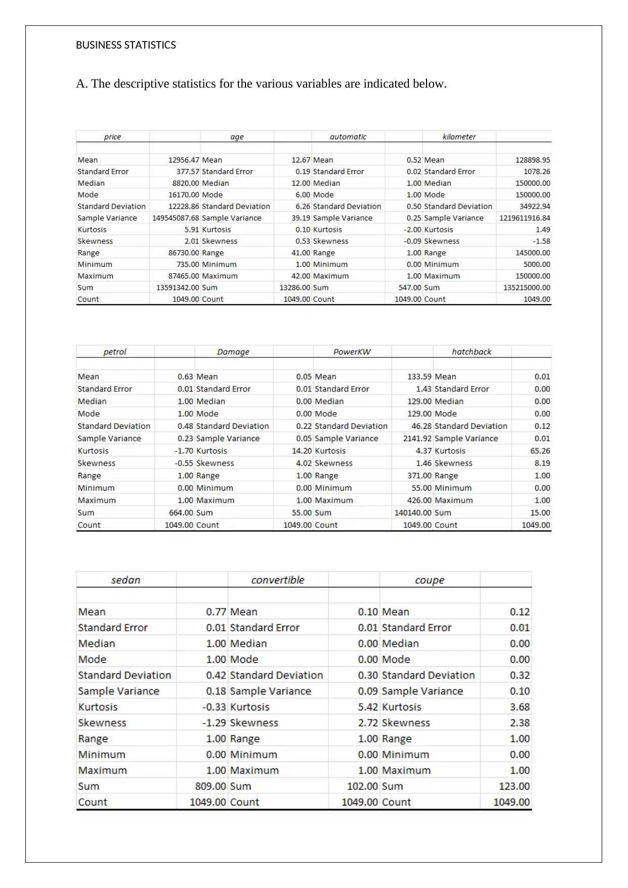
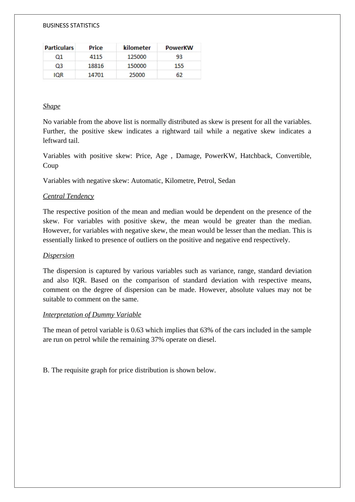
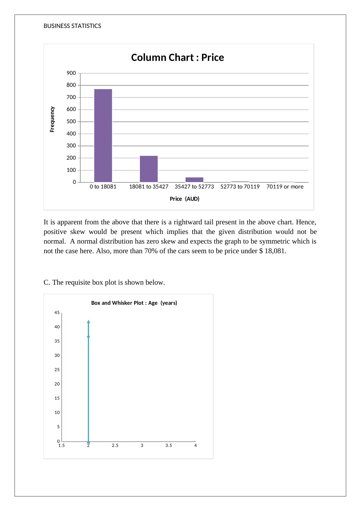
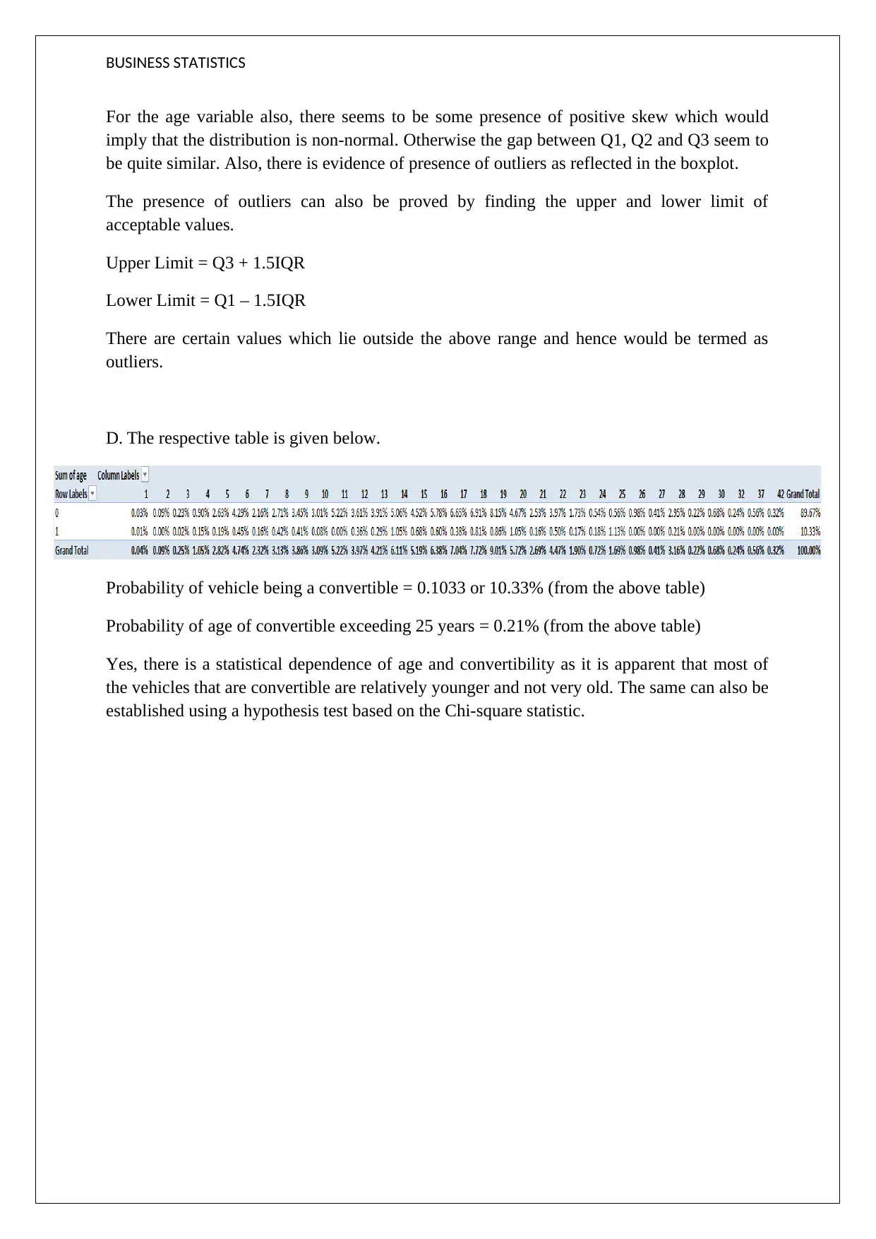
The homework assignment delves into the descriptive statistics of various business-related variables, highlighting their distribution characteristics. It explains that none of the listed variables follow a normal distribution due to the presence of skewness, which is either positive or negative indicating rightward or leftward tails respectively. The analysis includes central tendency measures where mean and median positions are discussed in relation to skewness, dispersion metrics like variance and standard deviation, and interpretations involving dummy variables such as car fuel types. Graphical representations including price distribution graphs and box plots illustrate skewness and outliers, reinforcing the statistical findings with calculations of upper and lower limits for outlier identification. The assignment concludes by examining probabilities related to vehicle characteristics, like convertibility, showing dependence between age and convertibility through a Chi-square hypothesis test.

BUSINESS STATISTICS
A. The descriptive statistics for the various variables are indicated below.

BUSINESS STATISTICS
Shape
No variable from the above list is normally distributed as skew is present for all the variables.
Further, the positive skew indicates a rightward tail while a negative skew indicates a
leftward tail.
Variables with positive skew: Price, Age , Damage, PowerKW, Hatchback, Convertible,
Coup
Variables with negative skew: Automatic, Kilometre, Petrol, Sedan
Central Tendency
The respective position of the mean and median would be dependent on the presence of the
skew. For variables with positive skew, the mean would be greater than the median.
However, for variables with negative skew, the mean would be lesser than the median. This is
essentially linked to presence of outliers on the positive and negative end respectively.
Dispersion
The dispersion is captured by various variables such as variance, range, standard deviation
and also IQR. Based on the comparison of standard deviation with respective means,
comment on the degree of dispersion can be made. However, absolute values may not be
suitable to comment on the same.
Interpretation of Dummy Variable
The mean of petrol variable is 0.63 which implies that 63% of the cars included in the sample
are run on petrol while the remaining 37% operate on diesel.
B. The requisite graph for price distribution is shown below.

BUSINESS STATISTICS
0 to 18081 18081 to 35427 35427 to 52773 52773 to 70119 70119 or more
0
100
200
300
400
500
600
700
800
900
Column Chart : Price
Price (AUD)
Frequency
It is apparent from the above that there is a rightward tail present in the above chart. Hence,
positive skew would be present which implies that the given distribution would not be
normal. A normal distribution has zero skew and expects the graph to be symmetric which is
not the case here. Also, more than 70% of the cars seem to be price under $ 18,081.
C. The requisite box plot is shown below.
1.5 2 2.5 3 3.5 4
0
5
10
15
20
25
30
35
40
45
Box and Whisker Plot : Age (years)

BUSINESS STATISTICS
For the age variable also, there seems to be some presence of positive skew which would
imply that the distribution is non-normal. Otherwise the gap between Q1, Q2 and Q3 seem to
be quite similar. Also, there is evidence of presence of outliers as reflected in the boxplot.
The presence of outliers can also be proved by finding the upper and lower limit of
acceptable values.
Upper Limit = Q3 + 1.5IQR
Lower Limit = Q1 – 1.5IQR
There are certain values which lie outside the above range and hence would be termed as
outliers.
D. The respective table is given below.
Probability of vehicle being a convertible = 0.1033 or 10.33% (from the above table)
Probability of age of convertible exceeding 25 years = 0.21% (from the above table)
Yes, there is a statistical dependence of age and convertibility as it is apparent that most of
the vehicles that are convertible are relatively younger and not very old. The same can also be
established using a hypothesis test based on the Chi-square statistic.