Holmes Institute HI6007 Statistics Group Assignment, T1 2019

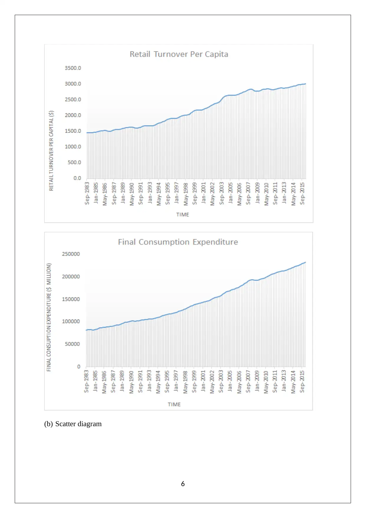
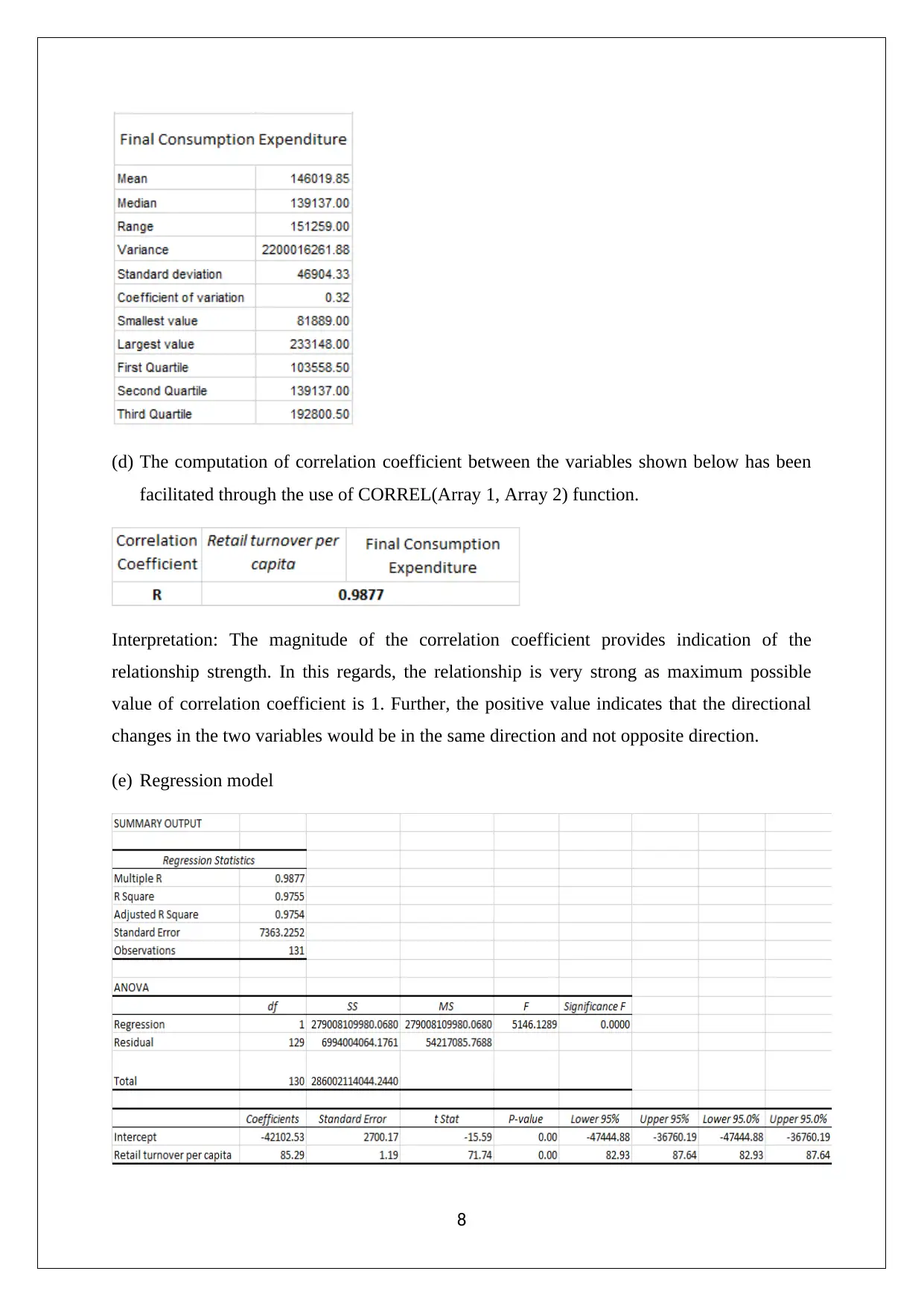
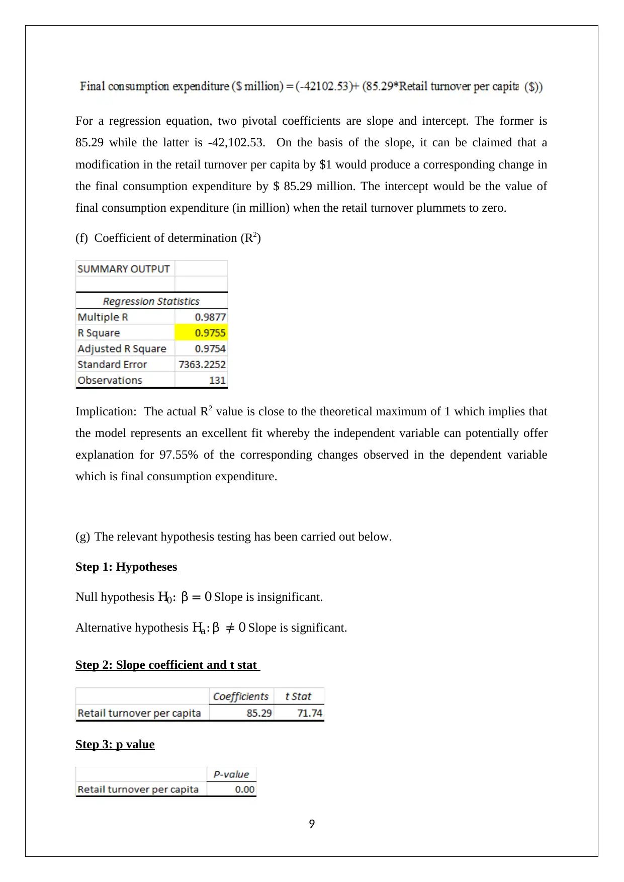
This document provides a complete solution to a statistics assignment, addressing various aspects of data analysis and interpretation. The assignment covers a range of topics, including the analysis of Australian export values using column charts and percentage distributions, frequency and cumulative frequency distributions of umbrella sales, and the creation of histograms and ogives. It further delves into time series analysis, scatter diagrams, and descriptive statistics. A significant portion of the solution is dedicated to regression analysis, including the computation and interpretation of the correlation coefficient, the construction of a regression model, and the analysis of its coefficients (slope, intercept, and coefficient of determination). The solution also includes hypothesis testing to determine the significance of the slope and the linear relationship between variables. The assignment incorporates the use of Excel functions for calculations and the interpretation of statistical outputs, such as standard error and p-values, to draw meaningful conclusions about the data and the relationships between variables. The assignment is based on the data provided in the assignment brief and is solved step by step.

STATISTICS
STUDENT ID:
[Pick the date]

Question 1
(a) Australian exports values for financial year 2004/05 and 2014/15 are exhibited through a
column chart.
(b) The expression of the Australian exports by destination in percentage terms is illustrated
below.
2

(c) The graphical illustrations of the destination distribution of Australian exports in 2004-
2005 and 2014-2015 point towards certain key trends.
 Barring China which has managed to enhance its share significantly, all the other
destinations considered have lost share in the Australia exports from 2004-2005 to
2014-2015. One of the key reasons for the same is the rapid rise in China as the
preferred destination for exports from Australia.
 It is quite strange that while exports to China have seen stupendous increase in
absolute terms, the exports to New Zealand have languished at the level of 2004-
2005 even in 2014-2015. Also, there is one destination namely United Kingdom
where during the period, absolute exports have dwindled from Australia.
Question 2
(a) Frequency distribution table pertaining to sale of umbrellas is displayed below.
3

Classes Frequency Relative Frequency
30-40 2 0.05
40-50 4 0.10
50-60 8 0.20
60-70 11 0.28
70-80 8 0.20
80-90 5 0.13
90-100 2 0.05
(b) Cumulative frequency distribution table pertaining to sale of umbrellas is displayed
below.
Classes Cumulative Frequency Cumulative Relative Frequency
30-40 2 0.05
40-50 6 0.15
50-60 14 0.35
60-70 25 0.63
70-80 33 0.83
80-90 38 0.95
90-100 40 1.00
(c) Histogram
(d) Ogive
4

(e) Required proportion
Proportion of umbrella sold < than 60 = 0.05 + 0.10 + 0.20 = 0.35
(f) Required proportion
Proportion of umbrella sold > than 70 = 0.20 + 0.13 + 0.05 = 0.38
Question 3
(a) Line graph to represent the time series
5

(b) Scatter diagram
6

The scatter plot above takes into consideration retail turnover per capita as the independent
variable which would determine the value of final consumption expenditure as the dependent
variable. This choice can be justified by highlighting the retail turnover is one of the key
determinants of consumption related expenditure.
(c) Descriptive statistics
7

(d) The computation of correlation coefficient between the variables shown below has been
facilitated through the use of CORREL(Array 1, Array 2) function.
Interpretation: The magnitude of the correlation coefficient provides indication of the
relationship strength. In this regards, the relationship is very strong as maximum possible
value of correlation coefficient is 1. Further, the positive value indicates that the directional
changes in the two variables would be in the same direction and not opposite direction.
(e) Regression model
8

For a regression equation, two pivotal coefficients are slope and intercept. The former is
85.29 while the latter is -42,102.53. On the basis of the slope, it can be claimed that a
modification in the retail turnover per capita by $1 would produce a corresponding change in
the final consumption expenditure by $ 85.29 million. The intercept would be the value of
final consumption expenditure (in million) when the retail turnover plummets to zero.
(f) Coefficient of determination (R2)
Implication: The actual R2 value is close to the theoretical maximum of 1 which implies that
the model represents an excellent fit whereby the independent variable can potentially offer
explanation for 97.55% of the corresponding changes observed in the dependent variable
which is final consumption expenditure.
(g) The relevant hypothesis testing has been carried out below.
Step 1: Hypotheses
Null hypothesis H0: β = 0 Slope is insignificant.
Alternative hypothesis Ha : β ≠ 0 Slope is significant.
Step 2: Slope coefficient and t stat
Step 3: p value
9

Step 4: Alpha
Significance level (Alpha) = 0.05
Step 5: Conclusion
p value is not higher than significance level and thereby rejection of H0 is warranted thereby
leading to acceptance of H1. This implies that both slope and linear relationship between
variables is significant.
(h) The standard error value has been identified from the regression output as shown below.
The above standard error is not large which is on expected lines considering the significance
of slope and high value of R2. All these collectively hint at the given simple regression model
being an excellent fit and resulting in minimal deviations between actual and predicted values
of the dependent variable.
10