Business Statistics Report: Seasonal Indexes and Business Decisions

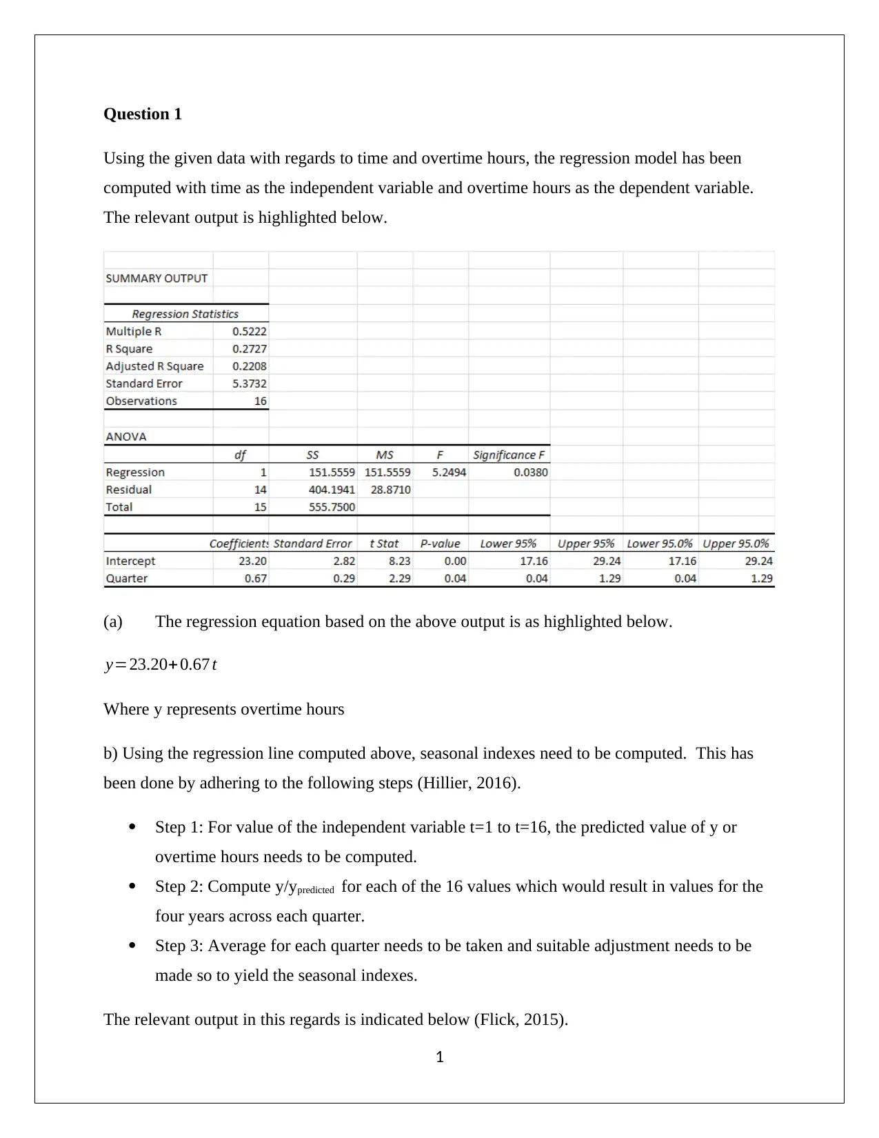
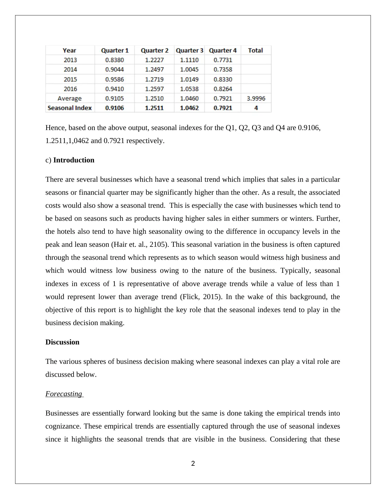
This business statistics report delves into the application of seasonal indexes and hypothesis testing within a business context. The report begins with a regression analysis of overtime hours, leading to the computation of seasonal indexes for different quarters. The core of the report explores the crucial role of seasonal indexes in various business decision-making spheres, including forecasting, capital projects, and the analysis of business performance. The report also includes a hypothesis test concerning exam scores, calculating z-statistics, p-values, and the probability of a Type II error. The report emphasizes the importance of these statistical tools in making informed business decisions and achieving accurate forecasting, particularly in industries with seasonal trends. The report concludes with a discussion on the practical implications of these statistical methods for business management.

BUSINESS STATISTICS
Student ID:
[Pick the date]

Question 1
Using the given data with regards to time and overtime hours, the regression model has been
computed with time as the independent variable and overtime hours as the dependent variable.
The relevant output is highlighted below.
(a) The regression equation based on the above output is as highlighted below.
y=23.20+ 0.67 t
Where y represents overtime hours
b) Using the regression line computed above, seasonal indexes need to be computed. This has
been done by adhering to the following steps (Hillier, 2016).
 Step 1: For value of the independent variable t=1 to t=16, the predicted value of y or
overtime hours needs to be computed.
 Step 2: Compute y/ypredicted for each of the 16 values which would result in values for the
four years across each quarter.
 Step 3: Average for each quarter needs to be taken and suitable adjustment needs to be
made so to yield the seasonal indexes.
The relevant output in this regards is indicated below (Flick, 2015).
1

Hence, based on the above output, seasonal indexes for the Q1, Q2, Q3 and Q4 are 0.9106,
1.2511,1,0462 and 0.7921 respectively.
c) Introduction
There are several businesses which have a seasonal trend which implies that sales in a particular
seasons or financial quarter may be significantly higher than the other. As a result, the associated
costs would also show a seasonal trend. This is especially the case with businesses which tend to
be based on seasons such as products having higher sales in either summers or winters. Further,
the hotels also tend to have high seasonality owing to the difference in occupancy levels in the
peak and lean season (Hair et. al., 2105). This seasonal variation in the business is often captured
through the seasonal trend which represents as to which season would witness high business and
which would witness low business owing to the nature of the business. Typically, seasonal
indexes in excess of 1 is representative of above average trends while a value of less than 1
would represent lower than average trend (Flick, 2015). In the wake of this background, the
objective of this report is to highlight the key role that the seasonal indexes tend to play in the
business decision making.
Discussion
The various spheres of business decision making where seasonal indexes can play a vital role are
discussed below.
Forecasting
Businesses are essentially forward looking but the same is done taking the empirical trends into
cognizance. These empirical trends are essentially captured through the use of seasonal indexes
since it highlights the seasonal trends that are visible in the business. Considering that these
2

seasonal variations are inherent in the business and cannot be dispelled away with, it is
imperative to take these into consideration for any future forecasting of the business. It is
essential the future trends of business should consider these and capture them in forecasting so
that an accurate forecasting can be drawn. This plays a pivotal role in the management decision
making (Hastie, Tibshirani and Friedman, 2011).
Consider for instance, an ice-cream manufacturer whose business tends to seasonal with sales in
summers being 50% higher than the corresponding sales in winter. Assume that the company is
running at 100% capacity utilization and is able to match 100% sales demand in summers.
However, owing to the popularity the management estimates that in the future demand is
expected to grow further. In such a scenario, it is essential to take into consideration the seasonal
indexes so as to be able to forecast the summer sales accurately going ahead. This is because the
sales in the winter months would not pose a problem for the company as it already has a spare
capacity. Hence, based on incremental unmet demand in the future, the management of the
company would need to have suitable arrangements in place so that the business interests are
safeguarded (Hillier, 2016).
The case of the given steel mill can also be taken into consideration. The given data highlights
the overtime hours which essentially would be linked to the production of steel. Hence, it would
be fair to conclude that in the quarters when the overtime hours are more, the production of steel
would be also higher. The seasonal indexes for the Q1, Q2, Q3 and Q4 have been computed as
0.9106, 1.2511,1,0462 and 0.7921 respectively. Based on the above, it can be estimated that steel
production is highest in Q2 and is about 25% higher than the average production level. Further,
the lowest production of steel would be witnessed in Q4 where the steel production would be
21% lower than the average. Considering the differential overtime hours in different quarters, it
is essential that the manpower planning needs to be carried out using the above information.
Additionally, the manpower must also ensure that their availability corresponds to the seasonal
trends so that the business demands can be fulfilled (Hair et. al., 2015).
The forecasting using seasonal indexes is also quite helpful in considering the capital projects
particularly when the capacity utilisation is very high and hence additional capacities would have
to be set to cater to the incremental demand. These decisions cannot be undertaken without the
accurate forecasting of the future requirements of the business. Thus, the seasonal indexes play a
3

critical role in ensuring that the business can capitalise on the potential future growth in the most
cost efficient manner. Capitalising in the cost efficient manner is essential considering that
capacity expansion if often not the right choice considering that surplus demand is limited to
particular quarters only and thus the management needs to consider all options particularly
outsourcing manufacturing (Flick, 2015).
Analysis of business performance
The presence of seasonal trends can make it difficult to analyse the business as the rise and fall in
sales or profits can be attributed to the seasonal factors. Hence, it is essential to deseasonalise the
financial information so as to obtain the data which is free from the seasonal effects. This
information is easier to interpret and highlight the business trends based on empirical trends.
Further, any deviations from a general trend can also be interpreted in seasonal terms. This is
because the positive or negative performance of the business may be attributed to seasonal
factors which are external to the business and hence not in the control of the management. Based
on this, the management can assess the performance of not only the business but also the
underlying employees (Hastie, Tibshirani and Friedman, 2011).
Conclusion
On the basis of the above, it can be concluded that seasonal indexes provide vital information in
relation to the seasonal variation of the business. Further, it is imperative for the management to
consider this seasonal trend owing to the pivotal information that is contained which can help not
only in forecasting but also analysis of business trends. This information is critical in order to
take useful decisions with regards to the future of the business and other decisions regarding
capital investment especially for fulfilling the incremental demand expected in the future.
Question 3
(i) The relevant inputs required for hypothesis test are highlighted below.
Population standard deviation σ =125
Random sample n=25 scores
4

Averagex=1375
(a) In order to conduct the given hypothesis, the following hypotheses need to be taken into
consideration.
Null hypothesis Ho : μ=1300 i.e. the average score on an exam for University of Adelaide does
not differ from the national average of 1300.
Alternative hypothesis Ha : μ>1300 i.e. the average score on an exam for University of Adelaide
is higher than the national average of 1300.
(b) The value of test statistic needs to be computed.
It can be seen from the above that population standard deviation is given and therefore, the
distribution can be assumed to be normally distributed and hence, z statistic would be taken into
consideration as the relevant test statistics (Flick, 2015).
z= x−μ
¿ ¿
z= 1375−1300
125
√25
z=3
The value of z statistic comes out to be 3 and can be represented using the following graph.
5

(c) The p value needs to be computed so as to decide if the null hypothesis ought to be
rejected or not.
For right tailed hypothesis testing, the p value comes out to be 0.00135.
(d) Assumed level of significance = 5%
It can be seen from the above analysis that p value is lower than level of significance and
therefore, sufficient evidence is present to reject the null hypothesis and to accept the alternative
hypothesis. Therefore, the conclusion can be drawn that “average score on LSAT paper at the
university of Adelaide is significantly higher than the national average of 1300” (Eriksson and
Kovalainen, 2015).
(ii) Probability of type II error
Null hypothesis Ho : μ=50
Alternative hypothesis Ha : μ>50
And,
μ=55
σ =10
6

n=16
∝=0.05
Here, rejection region needs to be determined.
RR=¿
RR=
{ x : x > x−50
10
√ 16
>1.645
}
RR= { x : x> 54.1125 }
Now,
¿ P ¿
¿ P ( Z ←0.355 )
¿ 0.3612
Therefore, probability of type II error comes out to be 0.3612.
References
7

Eriksson, P. and Kovalainen, A. (2015) Quantitative methods in business research (3rd ed.).
London: Sage Publications.
Flick, U. (2015) Introducing research methodology: A beginner's guide to doing a research
project (4th ed.). New York: Sage Publications.
Hair, J. F., Wolfinbarger, M., Money, A. H., Samouel, P., and Page, M. J. (2015) Essentials of
business research methods (2nd ed.). New York: Routledge.
Hastie, T., Tibshirani, R. and Friedman, J. (2011) The Elements of Statistical Learning (4th
ed.). New York: Springer Publications.
Hillier, F. (2016) Introduction to Operations Research (6th ed.). New York: McGraw Hill
Publications.
8