Business Statistics Analysis Report: Version 1 Analysis - BUS11

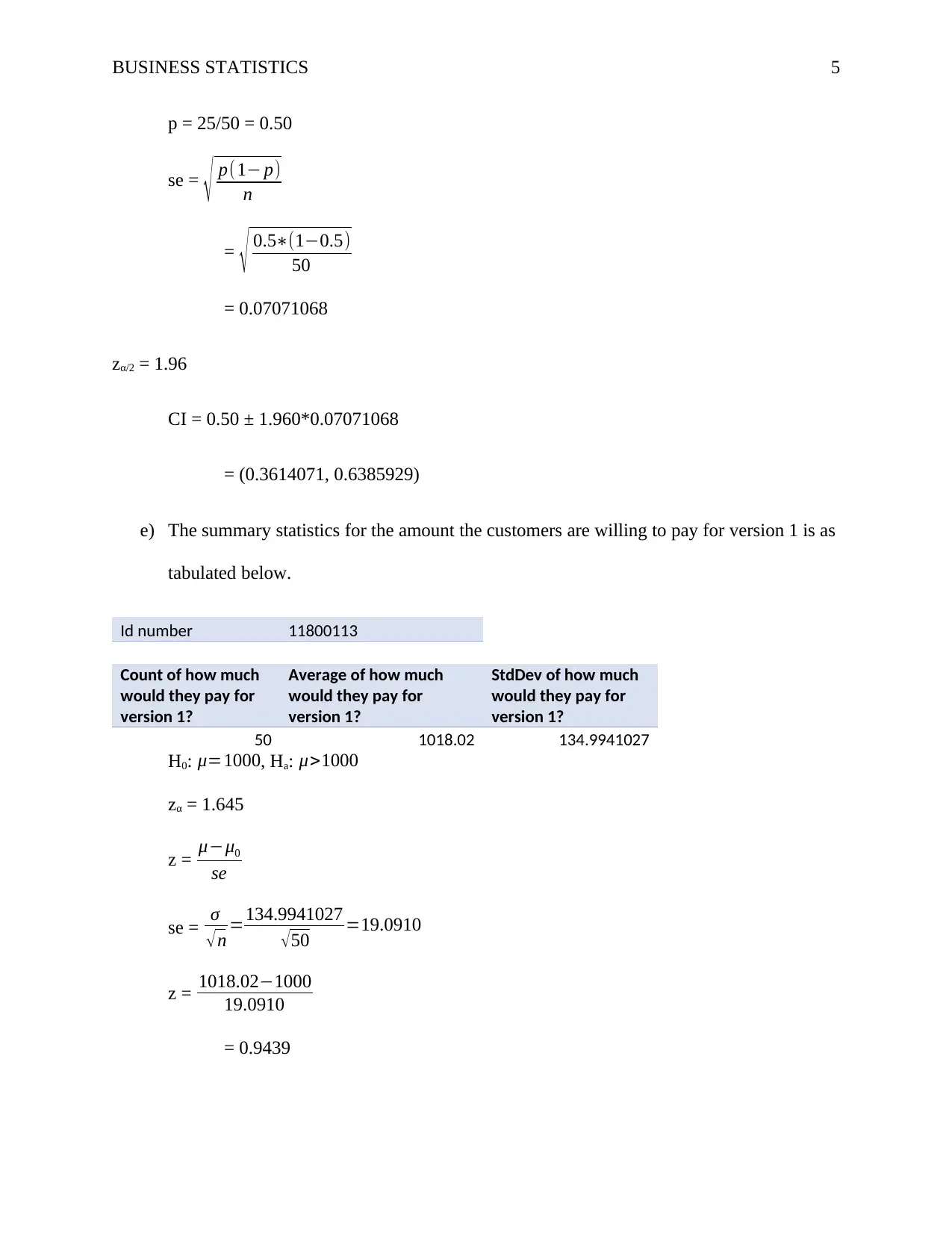
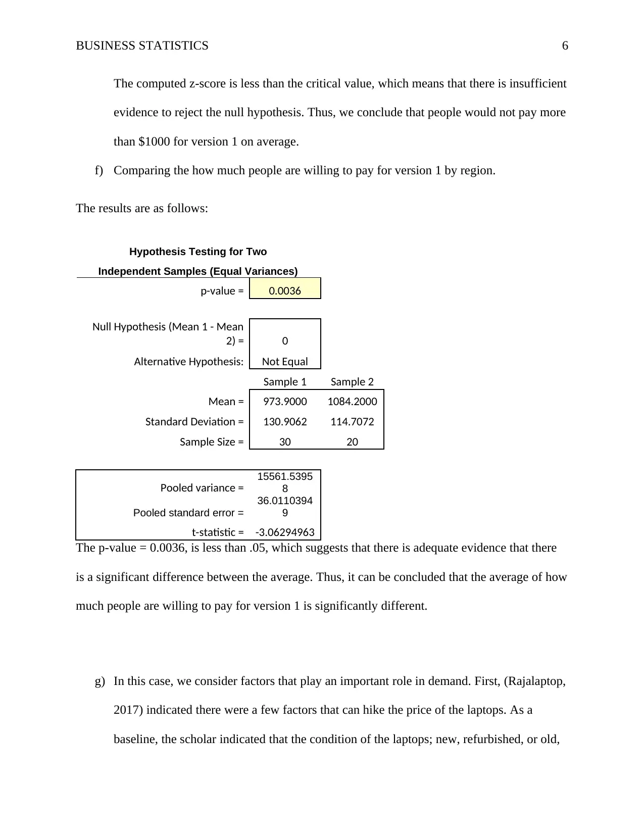
This report presents an analysis of a business statistics assignment focusing on customer preferences for laptop versions. The analysis investigates the relationship between customer region and the price they are willing to pay for version 1, revealing an average difference in willingness to pay between regions A and B. It examines the relationship between the price of version 1 and version 2, concluding a weak negative correlation. Further analysis explores the association between customer region and their willingness to pay more for version 1. The report tests the hypothesis about the average price customers are willing to pay for version 1. The report also identifies potential lurking variables, such as the presence of a university in a region, that could influence the relationship between variables and emphasizes the importance of considering such variables for accurate interpretations and generalizability of findings. The report also refers to factors that influence customer purchase habits such as the laptop's condition, weight, and specifications, along with after-sales services and the importance of R&D and differentiation in the product.

Running head: BUSINESS STATISTICS 1
Business Statistics
Name:
Institution

BUSINESS STATISTICS 2
a) The summary of the relationship between “what region” and “how much would they pay
for version 1” is as shown below.
Id number 11800113
Row Labels
Count of how much
would they pay for
version 1?
Average of how much
would they pay for
version 1?
StdDev of how much
would they pay for
version 1?
A 30 973.9 130.906218
B 20 1084.2 114.707225
Grand Total 50 1018 134.994103
The summary shows that on average those from region A are willing to pay $973.9 (SD =
$130.906218). On the other hand, those from region B were willing to pay $1084.2 (SD =
114.707225). The average difference is:
= 973.9 – 1084.2
= $-110.3
The customers from region 1 are $110.30 lower, the difference is not quite low and therefore, the
region is not a lurking variable.
b) The plot illustrating how much the customers are willing to pay for version 1 and version
2 is as shown below.

BUSINESS STATISTICS 3
$750 $850 $950 $1,050 $1,150 $1,250 $1,350
$750
$800
$850
$900
$950
$1,000
$1,050
$1,100
$1,150
$1,200
$1,250
f(x) = − 0.0628403715526313 x + 1076.09275504801
R² = 0.00530066672417684
how much would they pay for version 2?
How much would you pay for version 1
How much would you pay for version 2
The plot indicates that there is a weak negative relationship between the pay for version 1
and pay for version 2. The R-squared value is 0.0053, which shows a low proportion of
variation that can be accounted for by the fitted model. Thus, it can be concluded that
there is no relationship between how much one is willing to pay for version 1 and how
much they are willing to pay for version 2.
c) The summary of the relationship between “which region?” and “would you pay more for
version 1?” is as tabulated below.
Id number 11800113
Count of Would they pay more for version 1? Column Labels
Row Labels n y
Grand
Total
A 18 12 30
B 7 13 20
Grand Total 25 25 50

BUSINESS STATISTICS 4
Id number 11800113
Count of Would they pay more for version
1? Column Labels
Row Labels n y
Grand
Total
A 60.00%
40.00
% 100.00%
B 35.00%
65.00
% 100.00%
Grand Total 50.00%
50.00
% 100.00%
The summary shows that 40% of those who were from region A were willing to pay more
for version 1, whereas 65% from region B was willing to pay more.
The difference of the proportion is as follows:
p1 = 40.00% = 0.4000
p2 = 65.00% = 0.6500
p = p1 – p2 = 0.4000 – 0.6500
= -0.25
The results indicate that although a larger proportion of customers from region B are
willing to pay more for version 1. The proportion difference is not significant, which
means that the region of the customers is not a determinant whether they are willing to
pay more on version 1.
d) The 95% confidence interval for those willing to pay more on version 1, is as follows.
Id number 11800113
Column Labels
n y
Grand
Total
Count of Would they pay more for version 1? 25 25 50
95% CI = p ± zα/2 × se

BUSINESS STATISTICS 5
p = 25/50 = 0.50
se = √ p(1− p)
n
= √ 0.5∗(1−0.5)
50
= 0.07071068
zα/2 = 1.96
CI = 0.50 ± 1.960*0.07071068
= (0.3614071, 0.6385929)
e) The summary statistics for the amount the customers are willing to pay for version 1 is as
tabulated below.
Id number 11800113
Count of how much
would they pay for
version 1?
Average of how much
would they pay for
version 1?
StdDev of how much
would they pay for
version 1?
50 1018.02 134.9941027
H0: μ=1000, Ha: μ>1000
zα = 1.645
z = μ−μ0
se
se = σ
√ n =134.9941027
√ 50 =19.0910
z = 1018.02−1000
19.0910
= 0.9439

BUSINESS STATISTICS 6
The computed z-score is less than the critical value, which means that there is insufficient
evidence to reject the null hypothesis. Thus, we conclude that people would not pay more
than $1000 for version 1 on average.
f) Comparing the how much people are willing to pay for version 1 by region.
The results are as follows:
Hypothesis Testing for Two
Independent Samples (Equal Variances)
p-value = 0.0036
Null Hypothesis (Mean 1 - Mean
2) = 0
Alternative Hypothesis: Not Equal
Sample 1 Sample 2
Mean = 973.9000 1084.2000
Standard Deviation = 130.9062 114.7072
Sample Size = 30 20
Pooled variance = 15561.5395
8
Pooled standard error =
36.0110394
9
t-statistic = -3.06294963
The p-value = 0.0036, is less than .05, which suggests that there is adequate evidence that there
is a significant difference between the average. Thus, it can be concluded that the average of how
much people are willing to pay for version 1 is significantly different.
g) In this case, we consider factors that play an important role in demand. First, (Rajalaptop,
2017) indicated there were a few factors that can hike the price of the laptops. As a
baseline, the scholar indicated that the condition of the laptops; new, refurbished, or old,

BUSINESS STATISTICS 7
plays an important role. A new laptop is expected to cost more as it has a guarantee,
refurbished ones are a bit cheaper and they have been fixed a few defects. Also, the
weight of laptops is an important factor for the customers. A lighter laptop is quite
expensive compared to heavy laptops.
(Nasır, Yoruker, Güneş, & Ozdemi, 2007) on the other hand, indicated that in most cases,
customers purchasing laptops technically to update their laptops. Thus, the manufacturers
need first to identify to which base do their customers belong and try to update the
laptop's specification before taking one onto the market. Further, Nasir et al. (2007)
identified seven other factors that influence customers purchase habit. These factors
include; core technical issues such as processor speed, memory size etc.; connectivity and
mobility issues (i.e. Bluetooth, wireless, cam or TV/audio connections etc.); value-added
features (spill resistant keyboard, brand image, security etc.); after sales service
(guarantee, repairs and maintenance, warranty etc.); physical appearance (weight, color,
design etc.); peripheral devices (speakers, DVD/CD players, USB ports) and price.
If these seven conditions are met, the manufacturers will be able to reach the market and
increase the sale. In fact, the seller will be able to create an opportunity; since an
opportunity is where expectation meets demand. Lastly, the company should heavily
invest in R&D and create differentiation in their products.
h) Important explanatory/independent variables that escaped the attention of statistical
analyst are what should be referred to as lurking variables. Thus, diagnostic strategies
should be applied to identify the existence of the lurking variable. (Zachary, Lee, &
Iaccarino., 2019) stated that the lurking variable contains hidden information which
prevents a researcher to fully understanding the phenomenon of interest. Therefore, to

BUSINESS STATISTICS 8
understand the issue under investigation, the researcher should identify and consider them
to understand the phenomenon. As a strategy to identify the presence of lurking variable,
Zachary et al., (2019), suggested the use of dimensional analysis. This approach will
utilize Buckingham π theorem, which is used in computing dimensionless parameters
from a set of variables even when the form of an equation is unknown (Zohuri, 2017).
The presence of a lurking variable in a model can lead to misinterpretation of the
relationship between the variables. It can falsely inflate or deflate relationship between
variables. This fact, in most cases, is associated with low R-squared value or very large
R-squared value. As a remedy, Sullivan III, (2015) suggested a simpler strategy. First, the
researcher should try as much as possible to understand the process and factors that might
affect that process. Then, the statistician can plot the data and try to identify a nonlinear
trend which is associated with lurking variables.
When there exists a lurking variable, its changes lead to changes in both the dependent
and independent variable. This is normally regarded as causation. In the existence of
causation and well-established causal association, the results may not be generalized to
other population without such causal relationship (Sullivan III, 2015). In other words,
even when there is an established causal association, under different settings the causal
relationship may not hold. Also, when a causal relationship exists, it might be inadequate
to explain the relationship between the two variables. Therefore, it is quite important for
researchers to identify lurking variable if it exists, and determine their effect.
i) The summary statistics in part (f) indicated that the region was an important factor when
taking version 1 of the laptop to the market. Thus, it could be concluded that there was an
association between sales of laptop version 1 and the region of the customers. Also, from

BUSINESS STATISTICS 9
part (e) it was found that people were not willing to pay more than $1,000.00 on version
1. Further, it was found that there was no association between region and whether an
individual was willing to pay more for version 1. All these were factors that were thought
to affect the price the customers were willing to pay for a laptop. Which through the test
of hypothesis, a conclusion was reached either in favor or not in favor of the null
hypothesis.
As indicated in part (h) there might exist some lurking factors that might be attributed to
the existence of an association between variables. For instance, it was established that the
amount customers were willing to pay for version 1, was associated with the
region/location of the customer. However, there could be another factor which could lead
to such an association. As an example, consider a location where there is a university and
another state with no university. In the state with the university, it is expected that the
demand for laptops to be high, and customers willing to pay an even higher amount for
such a commodity. Thus, the existence of a university in a region is a lurking variable
which causes the relationship between the amount customers is willing to pay and region
to exist. Nonetheless, the existence of such an association cannot be generalized to all the
states. Thus, it is quite crucial to investigate whether there exists a lurking variable before
making any relational assessment on the data or at least understand all the factors that
might affect the response variable.

BUSINESS STATISTICS 10
References
Nasır, V. A., Yoruker, S., Güneş, F., & Ozdemi, Y. (2007). Factors influencing consumers’
Laptop Purchase. researchgate, 1-10.
Rajalaptop. (2017, 12 3). Some Factors that Affect your Laptop Price. Retrieved from
rajalaptop.com: https://rajalaptop.com/factors-affect-laptop-price/
Sullivan III, M. (2015). Fundamentals of statistics. Pearson.
Zachary, d. R., Lee, M., & Iaccarino., G. (2019). Lurking Variable Detection via Dimensional
Analysis. SIAM/ASA Journal on Uncertainty Quantification, 7(1), 232-259.
Zohuri, B. (2017). Dimensional analysis beyond the Pi theorem. Berlin: Springer.

BUSINESS STATISTICS 11