Business Statistics Assignment: Analysis, Probability, and Solutions

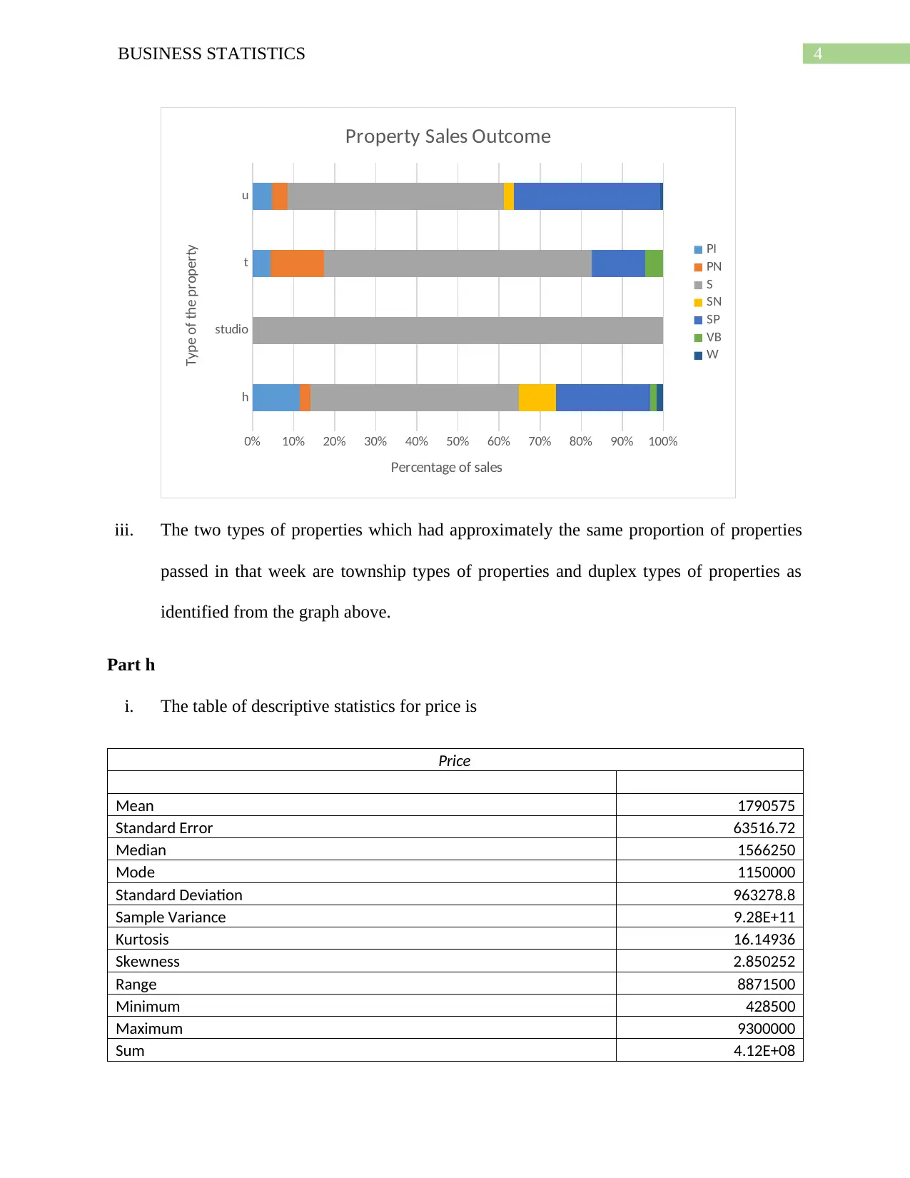
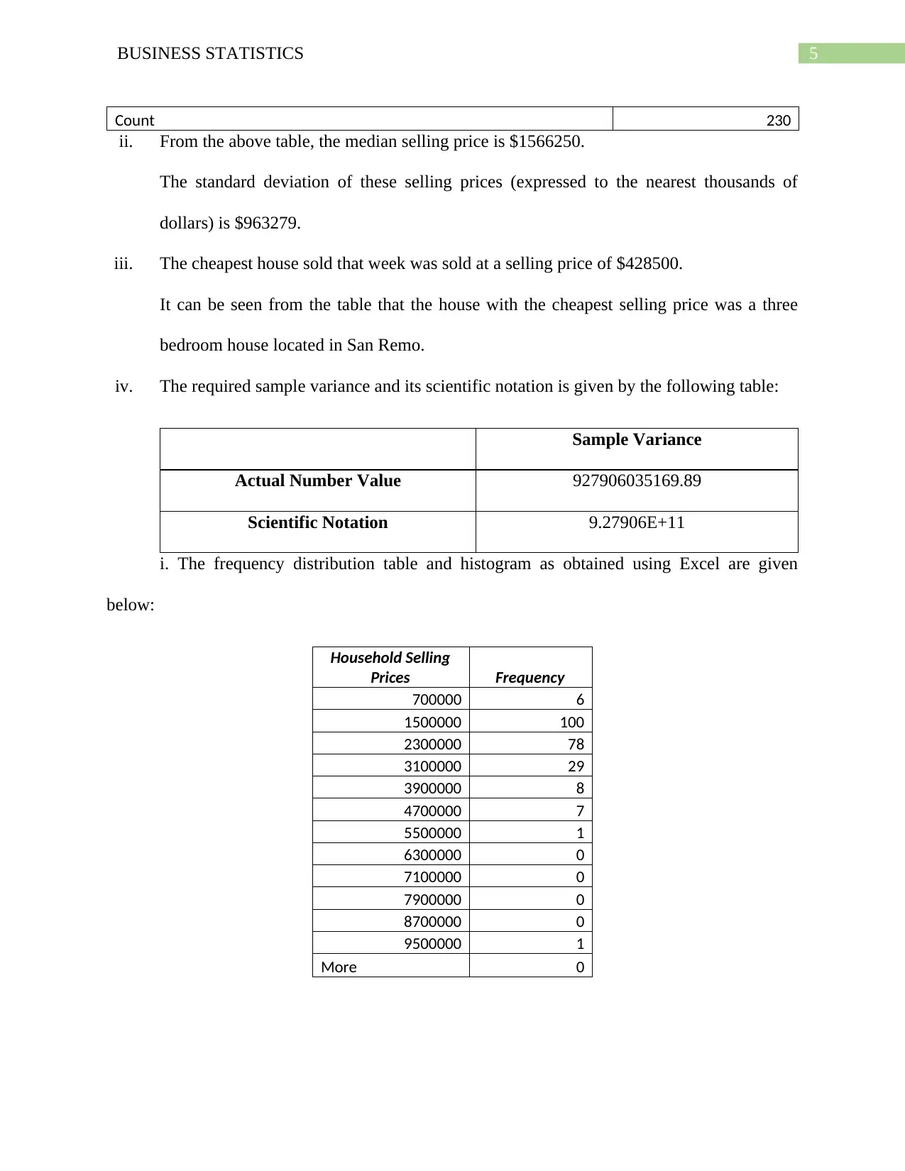
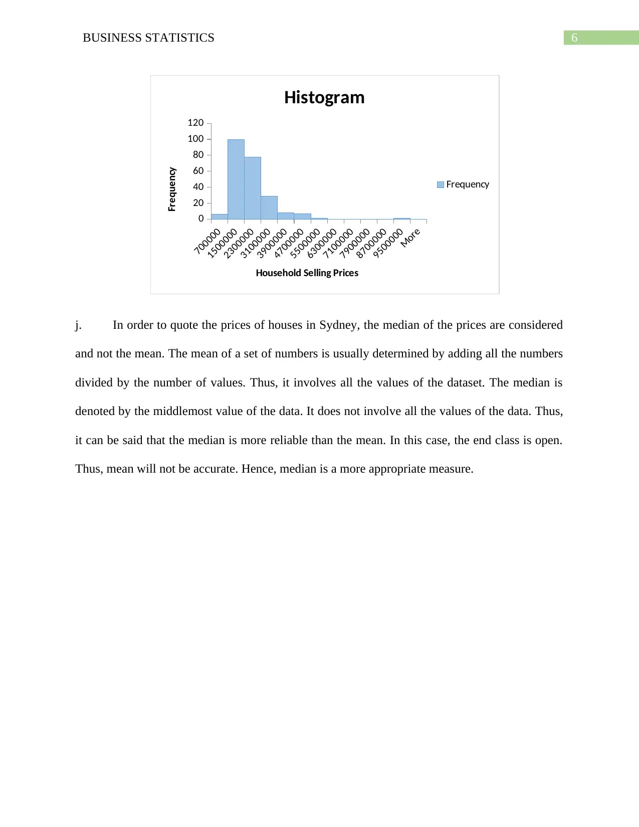
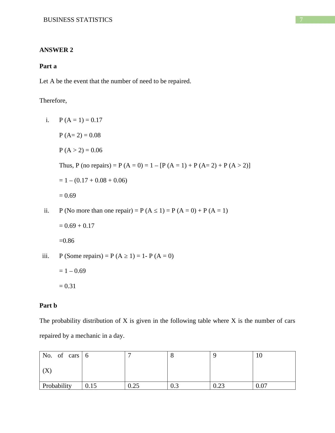
This business statistics assignment solution covers a range of topics, including data analysis, probability, and statistical distributions. The assignment begins with an analysis of qualitative and quantitative variables from a dataset, including identifying errors and calculating clearance rates for properties. It then delves into probability calculations using binomial and Poisson distributions, analyzing scenarios such as car repairs and emergency calls. Furthermore, the assignment explores normal distributions, calculating probabilities related to tire lifespan and customer satisfaction. The solution provides detailed explanations and calculations for each problem, including pivot tables, frequency distributions, and the application of statistical formulas. The assignment also provides a comparison between the mean and the median in quoting prices of houses in Sydney, as well as an analysis of the bias in a sample of people who watch movies. The document also includes the application of probability trees and the analysis of the independence of events. The solution encompasses a wide array of statistical concepts, offering a comprehensive understanding of the subject matter.

Running Head: BUSINESS STATISTICS
Business Statistics
Name of the Student
Name of the University
Author Note

1BUSINESS STATISTICS
ANSWER 1
Part a
i. Variables from the dataset, which are Qualitative and Normal, are Suburb,
Address, Type, Result and Agent.
ii. There are no variables in the dataset, which are both Qualitative and Normal.
iii. Variable from the dataset, which is Quantitative and ratio is price.
iv. The variable from the dataset, which is both Quantitative and Ordinal, is bedroom.
Part b
Result Code Overall Outcome
PI, NB, VB Property not sold
SP, PN Property sold prior to auction
S, SN Property sold at auction
SA, SS Property sold after auction
W Withdrawn from auction
Part c
i. By Suburb and Address, the four properties where the number of bedrooms is
missing is shown by the following table:
Suburb Address
Darlington 9/299 Abercrombie St.
Kirribilli 49/20 Carabella St.
Manly 1/19-23 Pittwater Rd.
North Sydney 307/54 High St.

2BUSINESS STATISTICS
ii. The properties which are errors, from the above identified properties are given as
follows:
Suburb Address Bedrooms Type Price Result Agent
Darlington 9/299 Abercrombie St u N/A PN Blues Point R
North Sydney 307/54 High St u N/A PN Blues Point R
These two properties are the errors because the price of the property is missing in
both the cases and both of the properties were sold before auction. Thus, these two
properties do not have any records during the auction.
Part d
Part e
i. It can be seen from the pivot table that there were 467 properties, which was listed for
auction in that day.

3BUSINESS STATISTICS
ii. The total number of properties that were sold that day (at auction, prior or after) is 244 +
31 + 121 = 396.
iii. The percentage of the number of properties sold at auction is = 396/467 = 84.8%.
Part f
i. The number of four bedroom houses listed for the auction that day is 106. These include
102 houses, 4 duplex and 1 townhouse.
ii. Out of these 106 houses, 91 were sold at the auction, prior or after.
iii. The percentage of the number of four bedroom houses sold (at the auction, prior or after)
is 91/106 = 85.8%
iv. Of all the listed properties, the clearance rate is 84.8% and for the four bedroom houses,
the clearance rate is 85.8%. Thus, it can be said the rate of clearance for the four bedroom
houses is better than the rate of clearance of all the properties overall for that week.
Part g
i. The two way pivot table for type by result is given below:
ii. The single horizontal component chart is given below:

4BUSINESS STATISTICS
h
studio
t
u
0% 10% 20% 30% 40% 50% 60% 70% 80% 90% 100%
Property Sales Outcome
PI
PN
S
SN
SP
VB
W
Percentage of sales
Type of the property
iii. The two types of properties which had approximately the same proportion of properties
passed in that week are township types of properties and duplex types of properties as
identified from the graph above.
Part h
i. The table of descriptive statistics for price is
Price
Mean 1790575
Standard Error 63516.72
Median 1566250
Mode 1150000
Standard Deviation 963278.8
Sample Variance 9.28E+11
Kurtosis 16.14936
Skewness 2.850252
Range 8871500
Minimum 428500
Maximum 9300000
Sum 4.12E+08

5BUSINESS STATISTICS
Count 230
ii. From the above table, the median selling price is $1566250.
The standard deviation of these selling prices (expressed to the nearest thousands of
dollars) is $963279.
iii. The cheapest house sold that week was sold at a selling price of $428500.
It can be seen from the table that the house with the cheapest selling price was a three
bedroom house located in San Remo.
iv. The required sample variance and its scientific notation is given by the following table:
Sample Variance
Actual Number Value 927906035169.89
Scientific Notation 9.27906E+11
i. The frequency distribution table and histogram as obtained using Excel are given
below:
Household Selling
Prices Frequency
700000 6
1500000 100
2300000 78
3100000 29
3900000 8
4700000 7
5500000 1
6300000 0
7100000 0
7900000 0
8700000 0
9500000 1
More 0

6BUSINESS STATISTICS
700000
1500000
2300000
3100000
3900000
4700000
5500000
6300000
7100000
7900000
8700000
9500000
More
0
20
40
60
80
100
120
Histogram
Frequency
Household Selling Prices
Frequency
j. In order to quote the prices of houses in Sydney, the median of the prices are considered
and not the mean. The mean of a set of numbers is usually determined by adding all the numbers
divided by the number of values. Thus, it involves all the values of the dataset. The median is
denoted by the middlemost value of the data. It does not involve all the values of the data. Thus,
it can be said that the median is more reliable than the mean. In this case, the end class is open.
Thus, mean will not be accurate. Hence, median is a more appropriate measure.

7BUSINESS STATISTICS
ANSWER 2
Part a
Let A be the event that the number of need to be repaired.
Therefore,
i. P (A = 1) = 0.17
P (A= 2) = 0.08
P (A > 2) = 0.06
Thus, P (no repairs) = P (A = 0) = 1 – [P (A = 1) + P (A= 2) + P (A > 2)]
= 1 – (0.17 + 0.08 + 0.06)
= 0.69
ii. P (No more than one repair) = P (A ≤ 1) = P (A = 0) + P (A = 1)
= 0.69 + 0.17
=0.86
iii. P (Some repairs) = P (A ≥ 1) = 1- P (A = 0)
= 1 – 0.69
= 0.31
Part b
The probability distribution of X is given in the following table where X is the number of cars
repaired by a mechanic in a day.
No. of cars
(X)
6 7 8 9 10
Probability 0.15 0.25 0.3 0.23 0.07

8BUSINESS STATISTICS
The mean number of cars repaired in a day is given by;
μ=∑ X i∗Pi
= (6*0.15) + (7*0.25) + (8*0.3) + (9*0.23) + (10*0.07)
= 7.82
= 8 [approx.]
The formula for calculating the standard deviation of the number of cars repaired in a day is
given by
√(∑ P i∗( X i−μ)2)
The necessary calculations to find out the standard deviation is given as follows:
No. cars X Probability Xi-μ (Xi-μ)^2 Pi*(Xi-μ)^2
6 0.15 -1.82 3.3124 19.8744
7 0.25 -0.82 0.6724 4.7068
8 0.3 0.18 0.0324 0.2592
9 0.23 1.18 1.3924 12.5316
10 0.07 2.18 4.7524 47.524
Total 1 0.9 10.162 84.896
The required standard deviation is √ 84.896=9.214=10(¿).
Part c
The sample that Paul selected is bias because
 The sample was drawn on the basis of the participation of the people of one particular
day. The result can vary a lot in the next day or the day after that. The number of people

9BUSINESS STATISTICS
watching the particular cinema today might not be the same on any other day. Thus, the
sample could have been collected for a week and not a day.
 Only female participants were considered in the sample. Considering only female
participants will not give a clear analysis of the frequency of people visiting the movies.
Part d
The table showing the members of Sydney golf club is given below:
Age Range Male Female Total
Under 18 55 23 78
18 to 30 165 45 201
31 to 50 300 90 390
Over 50 180 42 222
Total 900
i. The number of male members to be sampled from the age group of 31 to 50 years is
(300/900)*90 = 30.
ii. The number of female members to be sampled = (200/900)*90 = 20.

10BUSINESS STATISTICS
ANSWER 3
Part a
From the records of a company, it has been found out that four types of incidents are
described in the information. The events are, day shift workers, night shift workers, the workers
who turned up and workers who did not turn up.
Let the day shift workers be denoted as A and the workers who did not turn up be
denoted as B. Then, the night shift workers will be denoted as A and the workers who turned up
is denoted by B. The following diagram can give the probability tree containing the above
information.
The tree clearly states the following information:
P (A) = 0.7, P ( A) = 1 – 0.7 = 0.3

11BUSINESS STATISTICS
Again, P (B|D) = 0.2 P (B∨ A ¿ = 1 - 0.02 = 0.98.
Further, P (B/ A) = 0.04, P (B/ A ¿ = 1 – 0.04 = 0.96
Therefore, the percentage of day-shift workers who are not present on any given day = (0.7 *
0.2) * 100 = 1.4%
The percentage of night shift workers are absent on any given day = (0.3 * 0.4) * 100 = 1.2%
Therefore, the total percentage of workers who are absent on any given day = 1.4% + 1.2% =
2.6%
Part b
Absenteeism will be independent of the shift worked if P (B|A) = P (B). Here, this is not the
case. Therefore, absenteeism depends on the working shifts.
ANSWER 4
Part a
i. P (Z > 0.4)
= 1 – P (Z < 0.4)
= 1 – 0.6554
= 0.3466.
ii. P (-1.35 ≤ Z ≤ 1.25)
= P (Z ≤ 1.25) – P (Z ≤ -1.35)
= 0.8944 – 0.0885
=0.8059.