Business Statistics: Analyzing Real Estate Data - Assignment Solution

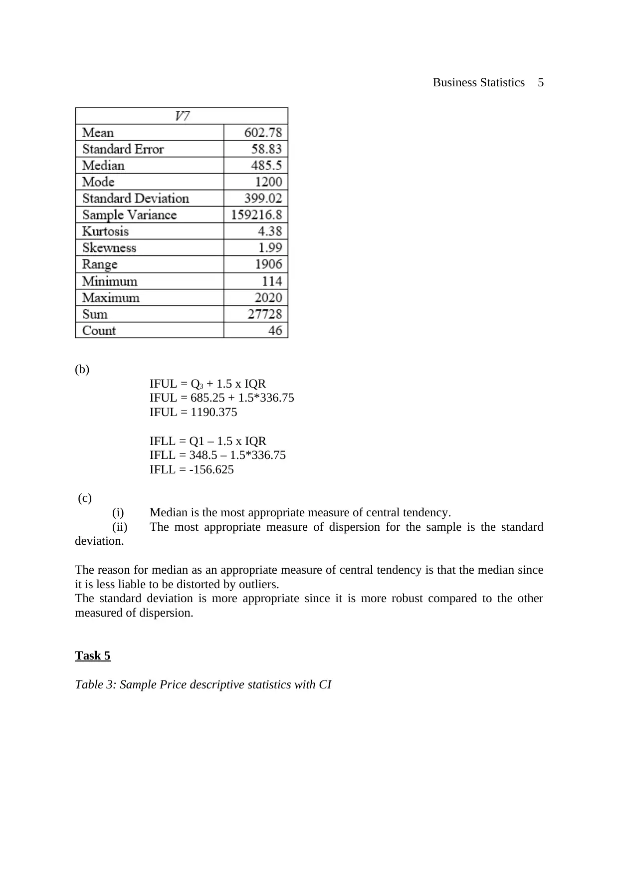
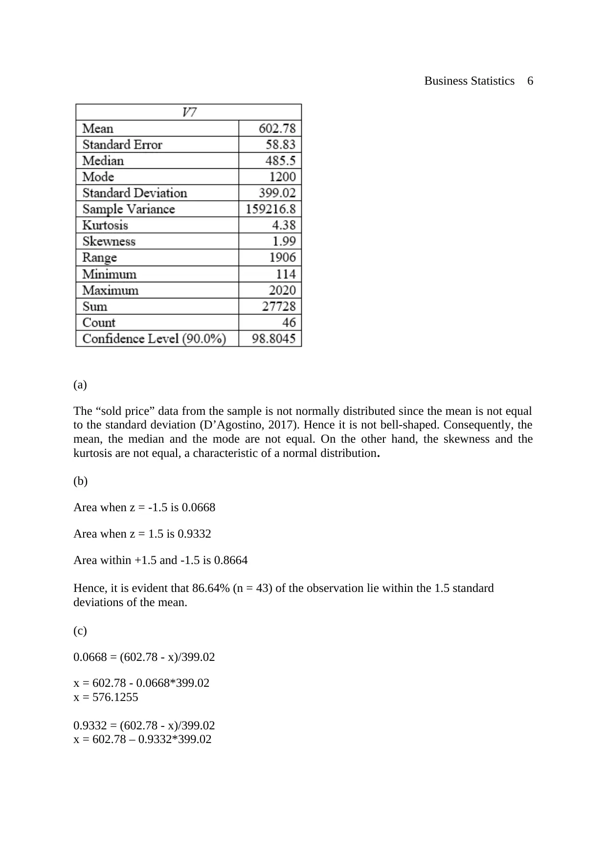
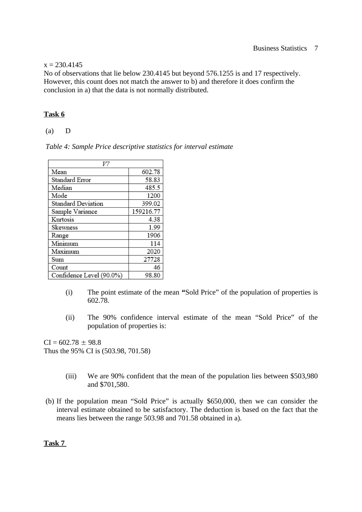
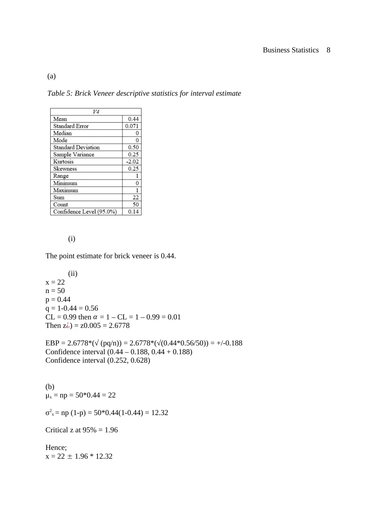
This business statistics assignment analyzes real estate data, covering various statistical concepts. It includes frequency charts and pie charts to visualize building types, sorted data tables of sold prices, and descriptive statistics calculations. The solution determines the 70th percentile, first and third quartiles, and interquartile range. It identifies the most appropriate measures of central tendency and dispersion and assesses data normality using the mean, standard deviation, skewness, and kurtosis. Confidence intervals are calculated for both the mean sold price and the proportion of brick veneer properties, with detailed explanations and references to statistical methods and formulas. The assignment provides a comprehensive overview of data analysis techniques, including interpreting results and drawing conclusions based on statistical evidence.

Running Header: Business Statistics 1
Business Statistics
Students name:
Student’s ID:
Institution:

Business Statistics 2
Task 1
As attached.
Task 2
Figure 1: Building Type Frequency Column Chart
Figure 2: Building Type Pie chart
(a) The number of properties in the sample consisting of brick buildings is 12.
(b) The brick veneer buildings (n = 12) occurs the most frequently in the sample.
(c) 22% (n = 11) of the properties in the sample consists of weatherboard buildings.

Business Statistics 3
Task 3
(a) Sorted “Sold Price” data
Table 1: Sorted sample “Sold Price”
PN Sold Price ($000s) Rank
192 114 1
278 190 2
193 230 3
10 239.5 4
371 265 5
344 295 6
362 305 7
119 310 8
347 323 9
300 330 10
79 340 11
86 347 12
342 353 13
110 375 14
92 410 15
396 420.5 16
301 432.5 17
5 435 18
330 441.5 19
207 445 20
171 465 21
61 476 22
334 481 23
227 490 24
120 491 25
379 518 26
240 525 27
144 552 28
15 563 29
228 596 30
351 600 31
146 615 32
356 618 33
262 641 34
23 700 35
281 711 36
183 724 37

Business Statistics 4
267 785 38
225 900 39
209 951 40
286 1060 41
394 1200 42
95 1200 43
223 1360 44
140 1885 45
248 2020 46
(b)
(i) 70th percentile.
Rank = (46+1)*( 70
100) = 32.9
70th Percentile is $618,000
(ii) The first and third quartiles.
First quartile = 348.5
Third quartile = 685.25
(c) At the 70th percentile, it is evident that 70% of the properties are cheaper than
&618,000 while 30% are pricier than $618,000.
(d)
Interquartile range = Q3 – Q1
= 685.25 – 348.5
= 336.75
It is evident that 25% of the prices are less than $348,500 while 25% of the properties cost
more than $685,250. The interquartile range is $336,750, which represents the range of the
middle 50% of the data.
Task 4
(a)
Table 2: Sample Price descriptive statistics

Business Statistics 5
(b)
IFUL = Q3 + 1.5 x IQR
IFUL = 685.25 + 1.5*336.75
IFUL = 1190.375
IFLL = Q1 – 1.5 x IQR
IFLL = 348.5 – 1.5*336.75
IFLL = -156.625
(c)
(i) Median is the most appropriate measure of central tendency.
(ii) The most appropriate measure of dispersion for the sample is the standard
deviation.
The reason for median as an appropriate measure of central tendency is that the median since
it is less liable to be distorted by outliers.
The standard deviation is more appropriate since it is more robust compared to the other
measured of dispersion.
Task 5
Table 3: Sample Price descriptive statistics with CI

Business Statistics 6
(a)
The “sold price” data from the sample is not normally distributed since the mean is not equal
to the standard deviation (D’Agostino, 2017). Hence it is not bell-shaped. Consequently, the
mean, the median and the mode are not equal. On the other hand, the skewness and the
kurtosis are not equal, a characteristic of a normal distribution.
(b)
Area when z = -1.5 is 0.0668
Area when z = 1.5 is 0.9332
Area within +1.5 and -1.5 is 0.8664
Hence, it is evident that 86.64% (n = 43) of the observation lie within the 1.5 standard
deviations of the mean.
(c)
0.0668 = (602.78 - x)/399.02
x = 602.78 - 0.0668*399.02
x = 576.1255
0.9332 = (602.78 - x)/399.02
x = 602.78 – 0.9332*399.02

Business Statistics 7
x = 230.4145
No of observations that lie below 230.4145 but beyond 576.1255 is and 17 respectively.
However, this count does not match the answer to b) and therefore it does confirm the
conclusion in a) that the data is not normally distributed.
Task 6
(a) D
Table 4: Sample Price descriptive statistics for interval estimate
(i) The point estimate of the mean “Sold Price” of the population of properties is
602.78.
(ii) The 90% confidence interval estimate of the mean “Sold Price” of the
population of properties is:
CI = 602.78  98.8
Thus the 95% CI is (503.98, 701.58)
(iii) We are 90% confident that the mean of the population lies between $503,980
and $701,580.
(b) If the population mean “Sold Price” is actually $650,000, then we can consider the
interval estimate obtained to be satisfactory. The deduction is based on the fact that the
means lies between the range 503.98 and 701.58 obtained in a).
Task 7

Business Statistics 8
(a)
Table 5: Brick Veneer descriptive statistics for interval estimate
(i)
The point estimate for brick veneer is 0.44.
(ii)
x = 22
n = 50
p = 0.44
q = 1-0.44 = 0.56
CL = 0.99 then α = 1 – CL = 1 – 0.99 = 0.01
Then z¿) = z0.005 = 2.6778
EBP = 2.6778*(√ (pq/n)) = 2.6778*(√(0.44*0.56/50)) = +/-0.188
Confidence interval (0.44 – 0.188, 0.44 + 0.188)
Confidence interval (0.252, 0.628)
(b)
μx = np = 50*0.44 = 22
σ2x = np (1-p) = 50*0.44(1-0.44) = 12.32
Critical z at 95% = 1.96
Hence;
x = 22  1.96 * 12.32

Business Statistics 9
x = (-2.15, 46.15)
(b)
The confidence interval for the population based on a) is 0.44  0.14. Thus, the confidence
interval at 95% is (0.3, 0.58).
It is evident that the intervals are not equal. It should be noted that the normal approximation
is not accurate especially for small values of n and should only be used when np ≥10 and np
(1-p) ≥10 (Soranzo & Epure, 2014). Thus, the direction of the change in precision should
always be expected.
Reference
D’Agostino, R. B. (2017). Tests for the normal distribution. In Goodness-of-fit-
techniques (pp. 367-420). Routledge.
Soranzo, A. and Epure, E., (2014). Very simply explicitly invertible approximations of
normal cumulative and normal quantile function. Applied Mathematical
Sciences, 8(87), pp.4323-4341.