GSBS6002 Business Analysis: Gloria Jones' Startup Café Project

This report presents a business analysis for Gloria Jones, who aspires to open her own café. The analysis addresses key factors like pricing, demographics, and location based on data collected from a survey of potential patrons. Ethical considerations were prioritized throughout the study. The findings suggest that customers are willing to pay more than $15 for a meal, with females showing a greater willingness to spend. While customers may not spend an average of $200 monthly on food, they are prepared to spend around $150. Zip codes 10, 11, and 12 are identified as promising locations due to higher spending expectations. The likelihood of patronizing the café varies with income levels. Finally, the average monthly food expenditure is correlated with meal price, age, and gender. The report uses statistical techniques like t-tests, ANOVA, and chi-square tests to validate hypotheses and provide actionable insights for Gloria Jones' startup.

RUNNING HEADER: GLORIA JONES BUSINESS ANALYSIS
1
Gloria Jones Business Analysis
Student’s name:
Student’s ID:
Institution:

Gloria Jones Business Analysis 2
Executive Summary
It is every wish for an entrepreneur to take charge of own self and start a business that will be a
route to independence. Gloria Jones always had this dream of having her own company. She
sought advice from her bank and was given the nod to pursue her dream as she had sufficient
saving from her job. However, she sought assistance to get informed advice on some of the
factors that she needs to consider.
The factors were on the basis of pricing, demographics, and location. Data were collected from a
sample of 2,000 individuals but only 400 responded. The ethical considerations had to be put
into consideration to ensure the study is pertinent to the rules of research.
The study found out that the potential patrons were ready to pay a worth for a meal that is higher
than $15. Moreover, there was a difference in the willingness to pay between males and females
as females were willing to spend more. However, Gloria should not anticipate all clients to
expend $200 monthly on average on food as they were ready to devote $150 on food monthly on
average. The zip code areas of 10, 11, and 12 provided the best location for the café as the
spending expectations were high. Subsequently, the prospect of patronizing the café differed
between people with dissimilar income levels. Finally, it was found out that the average people
devoted to food monthly could be described by the price on average people were prepared to pay
for meals, age, and gender.

Gloria Jones Business Analysis 3
Introduction
The following study aims to analyze some of the factors that should be considered before
establishing a start-up company. Gloria Jones is motivated by her dream to have her own café
one day. However, starting up a company comes with a myriad of challenges either personal or
financial (Stevenson & Jarillo, 2007).
Starting up a company is such a challenge. An individual who takes this path needs to be highly
motivated, with the will to accept work days which involve long hours and should be resilient
enough to bounce back from shortfalls which almost certainly occur (Davidson & Wiklund,
2007). Most people who are driven into such ventures need to keep in mind that they are starting
a company from ground level and building it (Sharma & Chrisma, 2007). Regardless of the
excitement of the risks versus the reward tradeoff, the startup ‘CEO’ needs to be proficient in all
aspects of the operations of the company which includes product development, marketing, and
finance.
The following study aims at tackling some of the issues and factors which Gloria Jones needs to
consider before setting up own café. Though she has a substantial capital from her savings from
her restaurant supply she is curious to get informed. To make the inform Gloria Jones about the
decisions she needs to make, the following research questions were developed:
Research questions
1. How much are potential patrons willing to pay for a meal? Is $15 a reasonable price? Is there a
difference in the willingness to pay between males and females?
2. Can Gloria expect all patrons to spend an average of $200 a month on food?

Gloria Jones Business Analysis 4
3. Which zip code area(s) provide the best location for the café? Does the expected average
monthly spend differ between potential patrons residing in different zip codes?
4. Does the likelihood to patronize the café differ between people with different income levels?
5. Can the average amount people spend on food each month be explained by the average price
people are willing to pay for meals, age, and gender?
Research Design
According to Bryman & Bell (2007), a research design is used in providing a framework that is
used in data analysis and data collection. There are three types of research designs which
include descriptive design, correlational design, experimental design and causal-comparative
design (Cresswell & Cresswell, 2017). The following study used a descriptive design, a
correlational design, and a causal-comparative design to test the various hypotheses.
A descriptive research design will be used to define the various characteristics of a variable.
They include the mean, standard deviation, the median and the mode (Shuttleworth, 2008). A
correlation design was also adapted to determine whether or not two or more variables are
correlated. On the other hand, a causal-comparative design is used to focus on the analysis of a a
specific problem so as to explain the pattern of relationship between variables.
When carrying out any research, it is paramount to gather the pertinent data which suits the
research design and the methodology. Data collection can either be primary or secondary.
According to Saunders (2011), primary data collection entails different methods such as
observation, survey, and focus groups. The following research made us of primary data. Data
were collected using questionnaires.

Gloria Jones Business Analysis 5
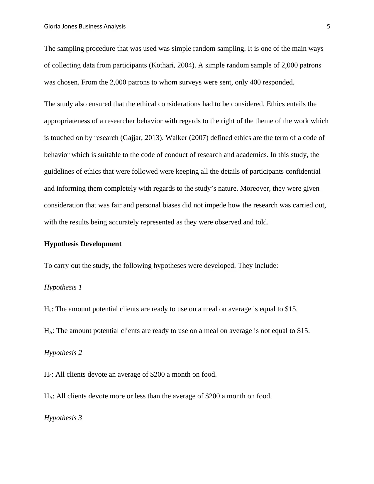
The sampling procedure that was used was simple random sampling. It is one of the main ways
of collecting data from participants (Kothari, 2004). A simple random sample of 2,000 patrons
was chosen. From the 2,000 patrons to whom surveys were sent, only 400 responded.
The study also ensured that the ethical considerations had to be considered. Ethics entails the
appropriateness of a researcher behavior with regards to the right of the theme of the work which
is touched on by research (Gajjar, 2013). Walker (2007) defined ethics are the term of a code of
behavior which is suitable to the code of conduct of research and academics. In this study, the
guidelines of ethics that were followed were keeping all the details of participants confidential
and informing them completely with regards to the study’s nature. Moreover, they were given
consideration that was fair and personal biases did not impede how the research was carried out,
with the results being accurately represented as they were observed and told.
Hypothesis Development
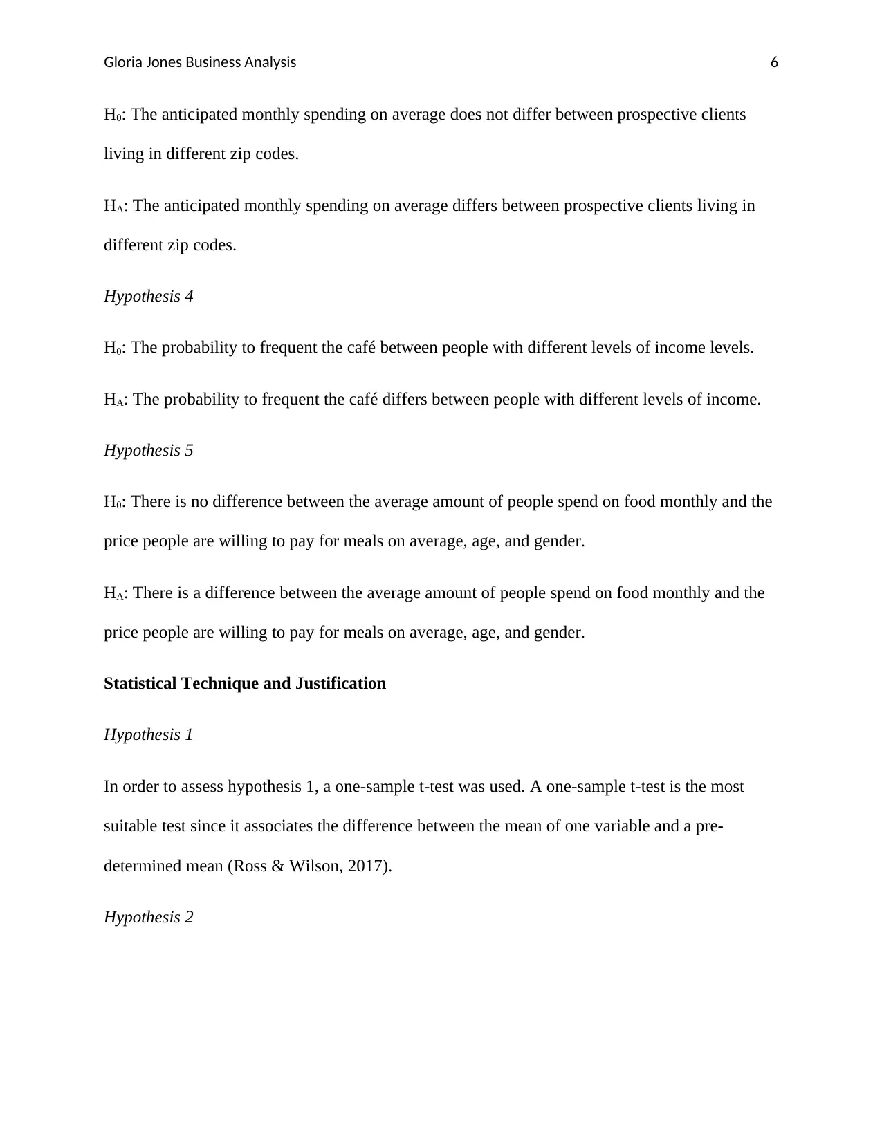
To carry out the study, the following hypotheses were developed. They include:
Hypothesis 1
H0: The amount potential clients are ready to use on a meal on average is equal to $15.
HA: The amount potential clients are ready to use on a meal on average is not equal to $15.
Hypothesis 2
H0: All clients devote an average of $200 a month on food.
HA: All clients devote more or less than the average of $200 a month on food.
Hypothesis 3

Gloria Jones Business Analysis 6
H0: The anticipated monthly spending on average does not differ between prospective clients
living in different zip codes.
HA: The anticipated monthly spending on average differs between prospective clients living in
different zip codes.
Hypothesis 4
H0: The probability to frequent the café between people with different levels of income levels.
HA: The probability to frequent the café differs between people with different levels of income.
Hypothesis 5
H0: There is no difference between the average amount of people spend on food monthly and the
price people are willing to pay for meals on average, age, and gender.
HA: There is a difference between the average amount of people spend on food monthly and the
price people are willing to pay for meals on average, age, and gender.
Statistical Technique and Justification
Hypothesis 1
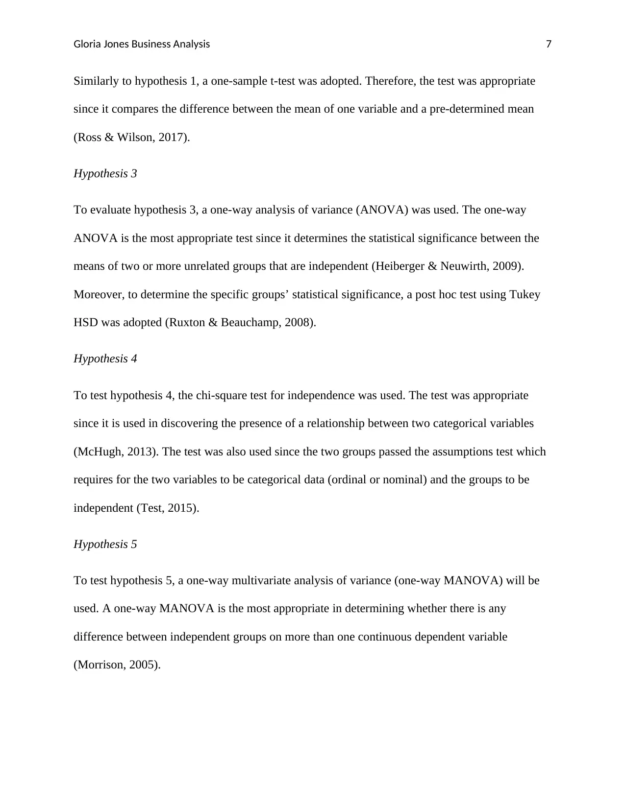
In order to assess hypothesis 1, a one-sample t-test was used. A one-sample t-test is the most
suitable test since it associates the difference between the mean of one variable and a pre-
determined mean (Ross & Wilson, 2017).
Hypothesis 2

Gloria Jones Business Analysis 7
Similarly to hypothesis 1, a one-sample t-test was adopted. Therefore, the test was appropriate
since it compares the difference between the mean of one variable and a pre-determined mean
(Ross & Wilson, 2017).
Hypothesis 3
To evaluate hypothesis 3, a one-way analysis of variance (ANOVA) was used. The one-way
ANOVA is the most appropriate test since it determines the statistical significance between the
means of two or more unrelated groups that are independent (Heiberger & Neuwirth, 2009).
Moreover, to determine the specific groups’ statistical significance, a post hoc test using Tukey
HSD was adopted (Ruxton & Beauchamp, 2008).
Hypothesis 4
To test hypothesis 4, the chi-square test for independence was used. The test was appropriate
since it is used in discovering the presence of a relationship between two categorical variables
(McHugh, 2013). The test was also used since the two groups passed the assumptions test which
requires for the two variables to be categorical data (ordinal or nominal) and the groups to be
independent (Test, 2015).
Hypothesis 5
To test hypothesis 5, a one-way multivariate analysis of variance (one-way MANOVA) will be
used. A one-way MANOVA is the most appropriate in determining whether there is any
difference between independent groups on more than one continuous dependent variable
(Morrison, 2005).

Gloria Jones Business Analysis 8
Results
Hypothesis 1
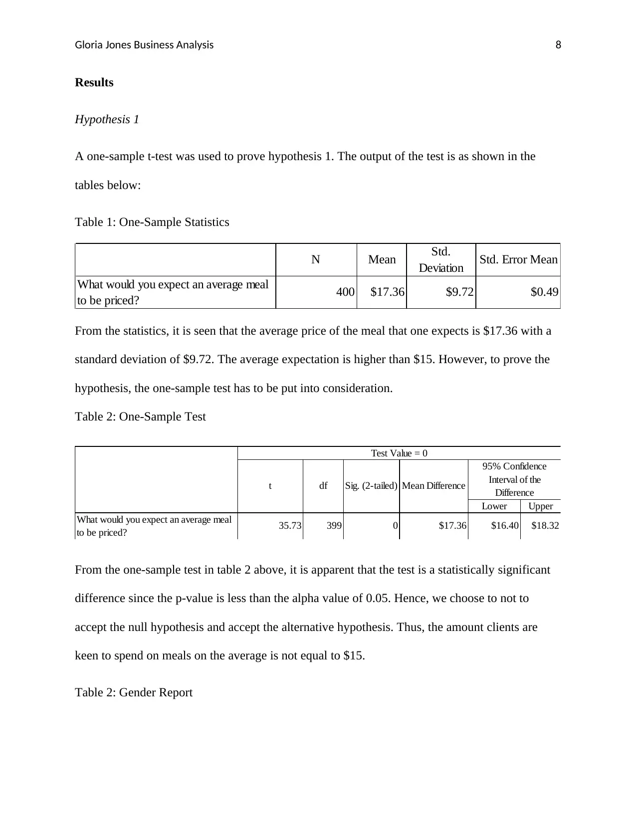
A one-sample t-test was used to prove hypothesis 1. The output of the test is as shown in the
tables below:
Table 1: One-Sample Statistics
N Mean Std.
Deviation Std. Error Mean
What would you expect an average meal
to be priced? 400 $17.36 $9.72 $0.49
From the statistics, it is seen that the average price of the meal that one expects is $17.36 with a
standard deviation of $9.72. The average expectation is higher than $15. However, to prove the
hypothesis, the one-sample test has to be put into consideration.
Table 2: One-Sample Test
Lower Upper
What would you expect an average meal
to be priced? 35.73 399 0 $17.36 $16.40 $18.32
Test Value = 0
t df Sig. (2-tailed) Mean Difference
95% Confidence
Interval of the
Difference
From the one-sample test in table 2 above, it is apparent that the test is a statistically significant
difference since the p-value is less than the alpha value of 0.05. Hence, we choose to not to
accept the null hypothesis and accept the alternative hypothesis. Thus, the amount clients are
keen to spend on meals on the average is not equal to $15.
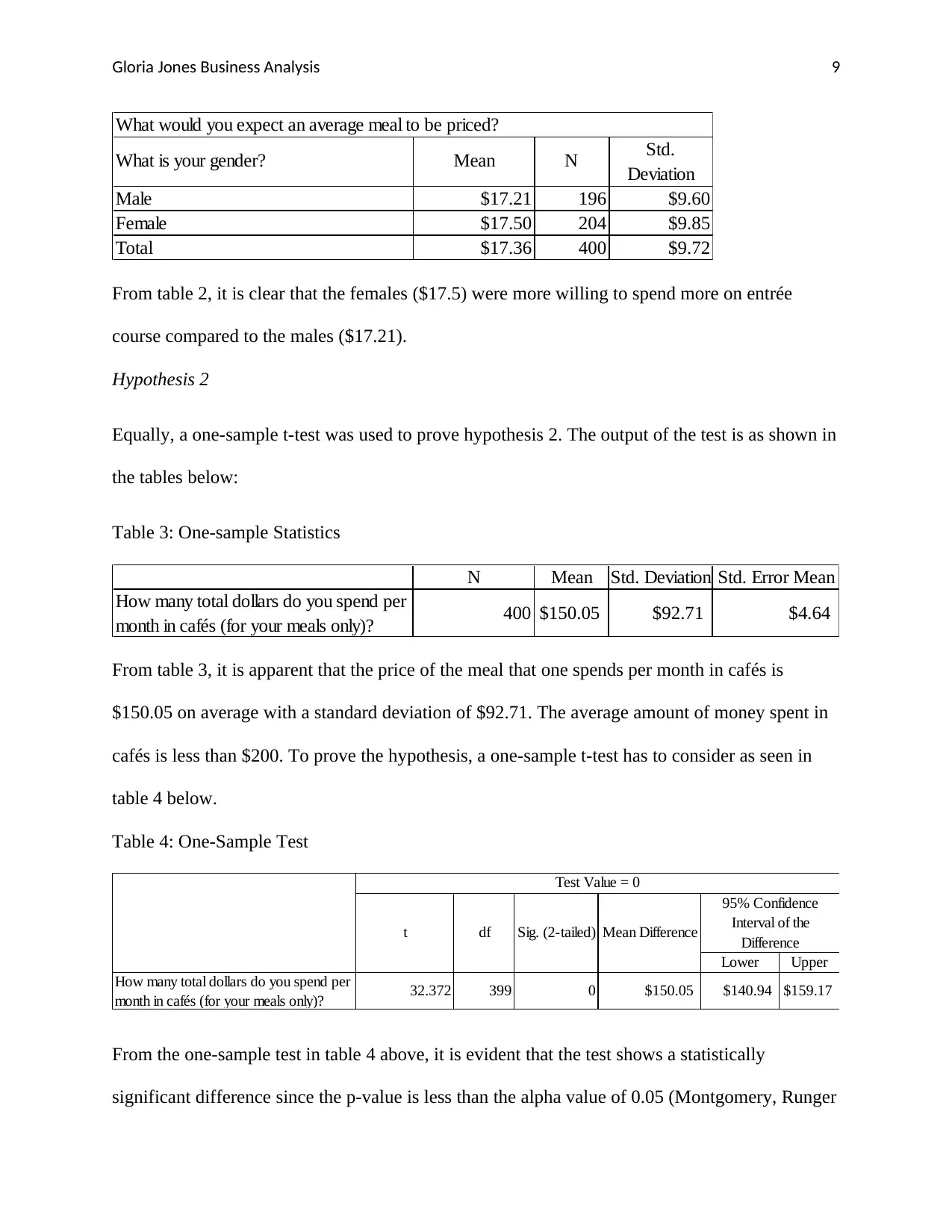
Table 2: Gender Report

Gloria Jones Business Analysis 9
What is your gender? Mean N Std.
Deviation
Male $17.21 196 $9.60
Female $17.50 204 $9.85
Total $17.36 400 $9.72
What would you expect an average meal to be priced?
From table 2, it is clear that the females ($17.5) were more willing to spend more on entrée
course compared to the males ($17.21).
Hypothesis 2
Equally, a one-sample t-test was used to prove hypothesis 2. The output of the test is as shown in
the tables below:
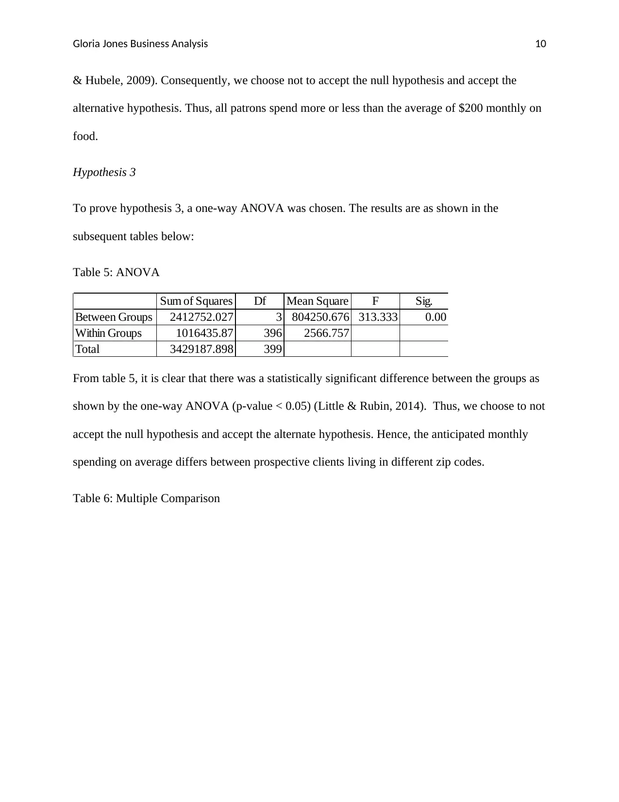
Table 3: One-sample Statistics
N Mean Std. Deviation Std. Error Mean
How many total dollars do you spend per
month in cafés (for your meals only)? 400 $150.05 $92.71 $4.64
From table 3, it is apparent that the price of the meal that one spends per month in cafés is
$150.05 on average with a standard deviation of $92.71. The average amount of money spent in
cafés is less than $200. To prove the hypothesis, a one-sample t-test has to consider as seen in
table 4 below.
Table 4: One-Sample Test
Lower Upper
How many total dollars do you spend per
month in cafés (for your meals only)? 32.372 399 0 $150.05 $140.94 $159.17
Test Value = 0
t df Sig. (2-tailed) Mean Difference
95% Confidence
Interval of the
Difference
From the one-sample test in table 4 above, it is evident that the test shows a statistically
significant difference since the p-value is less than the alpha value of 0.05 (Montgomery, Runger

Gloria Jones Business Analysis 10
& Hubele, 2009). Consequently, we choose not to accept the null hypothesis and accept the
alternative hypothesis. Thus, all patrons spend more or less than the average of $200 monthly on
food.
Hypothesis 3
To prove hypothesis 3, a one-way ANOVA was chosen. The results are as shown in the
subsequent tables below:
Table 5: ANOVA
Sum of Squares Df Mean Square F Sig.
Between Groups 2412752.027 3 804250.676 313.333 0.00
Within Groups 1016435.87 396 2566.757
Total 3429187.898 399
From table 5, it is clear that there was a statistically significant difference between the groups as
shown by the one-way ANOVA (p-value < 0.05) (Little & Rubin, 2014). Thus, we choose to not
accept the null hypothesis and accept the alternate hypothesis. Hence, the anticipated monthly
spending on average differs between prospective clients living in different zip codes.
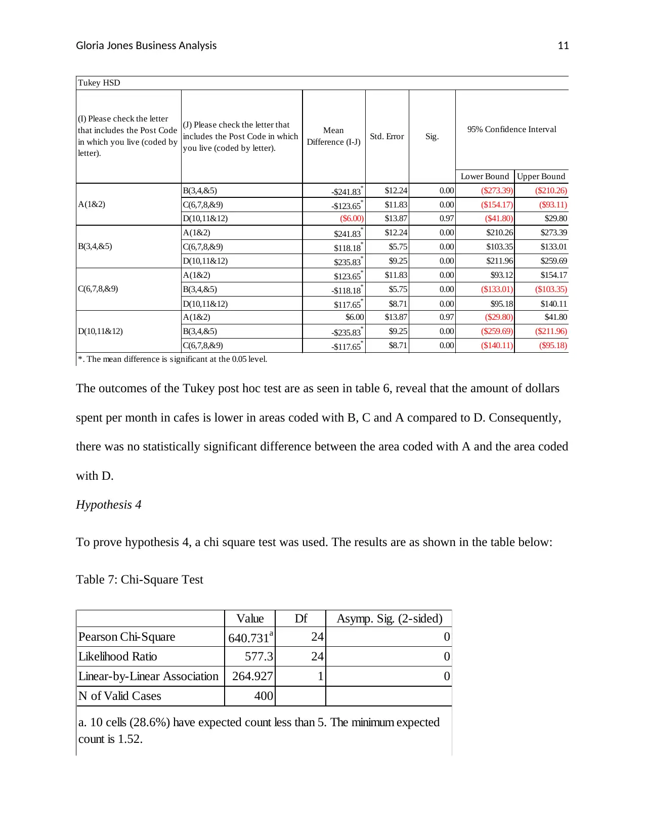
Table 6: Multiple Comparison

Gloria Jones Business Analysis 11
Lower Bound Upper Bound
B(3,4,&5) -$241.83* $12.24 0.00 ($273.39) ($210.26)
C(6,7,8,&9) -$123.65* $11.83 0.00 ($154.17) ($93.11)
D(10,11&12) ($6.00) $13.87 0.97 ($41.80) $29.80
A(1&2) $241.83* $12.24 0.00 $210.26 $273.39
C(6,7,8,&9) $118.18* $5.75 0.00 $103.35 $133.01
D(10,11&12) $235.83* $9.25 0.00 $211.96 $259.69
A(1&2) $123.65* $11.83 0.00 $93.12 $154.17
B(3,4,&5) -$118.18* $5.75 0.00 ($133.01) ($103.35)
D(10,11&12) $117.65* $8.71 0.00 $95.18 $140.11
A(1&2) $6.00 $13.87 0.97 ($29.80) $41.80
B(3,4,&5) -$235.83* $9.25 0.00 ($259.69) ($211.96)
C(6,7,8,&9) -$117.65* $8.71 0.00 ($140.11) ($95.18)
A(1&2)
B(3,4,&5)
C(6,7,8,&9)
D(10,11&12)
*. The mean difference is significant at the 0.05 level.
Tukey HSD
(I) Please check the letter
that includes the Post Code
in which you live (coded by
letter).
(J) Please check the letter that
includes the Post Code in which
you live (coded by letter).
Mean
Difference (I-J) Std. Error Sig. 95% Confidence Interval
The outcomes of the Tukey post hoc test are as seen in table 6, reveal that the amount of dollars
spent per month in cafes is lower in areas coded with B, C and A compared to D. Consequently,
there was no statistically significant difference between the area coded with A and the area coded
with D.
Hypothesis 4
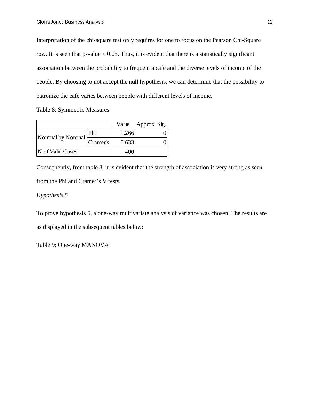
To prove hypothesis 4, a chi square test was used. The results are as shown in the table below:
Table 7: Chi-Square Test
Value Df Asymp. Sig. (2-sided)
Pearson Chi-Square 640.731a 24 0
Likelihood Ratio 577.3 24 0
Linear-by-Linear Association 264.927 1 0
N of Valid Cases 400
a. 10 cells (28.6%) have expected count less than 5. The minimum expected
count is 1.52.

Gloria Jones Business Analysis 12
Interpretation of the chi-square test only requires for one to focus on the Pearson Chi-Square
row. It is seen that p-value < 0.05. Thus, it is evident that there is a statistically significant
association between the probability to frequent a café and the diverse levels of income of the
people. By choosing to not accept the null hypothesis, we can determine that the possibility to
patronize the café varies between people with different levels of income.
Table 8: Symmetric Measures
Value Approx. Sig.
Phi 1.266 0
Cramer's V 0.633 0
400
Nominal by Nominal
N of Valid Cases
Consequently, from table 8, it is evident that the strength of association is very strong as seen
from the Phi and Cramer’s V tests.
Hypothesis 5
To prove hypothesis 5, a one-way multivariate analysis of variance was chosen. The results are
as displayed in the subsequent tables below:
Table 9: One-way MANOVA