Statistics Homework: Calculations, Graphing, and Data Interpretation

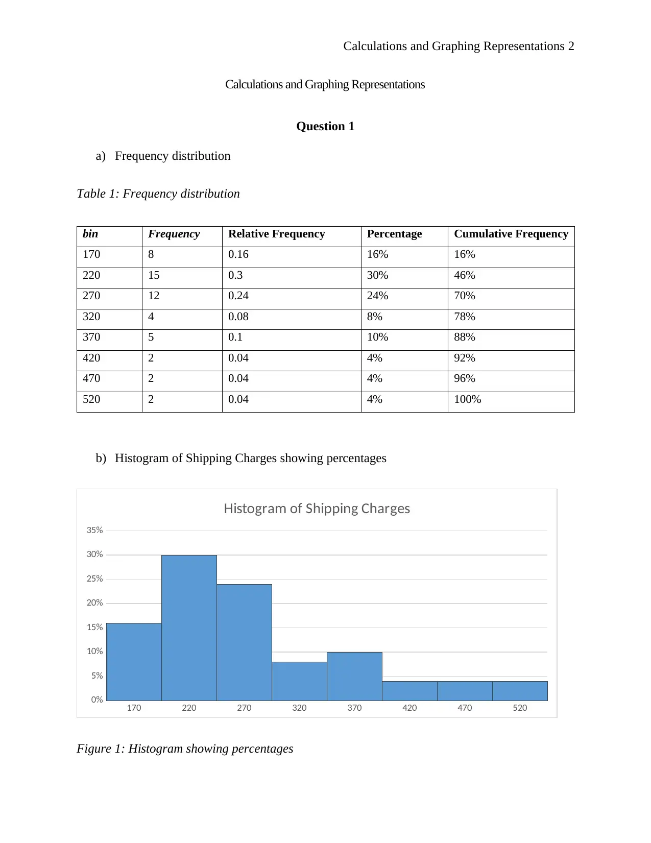
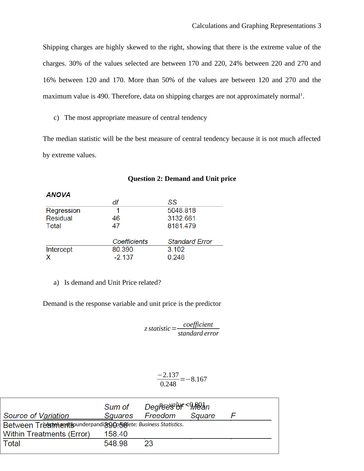
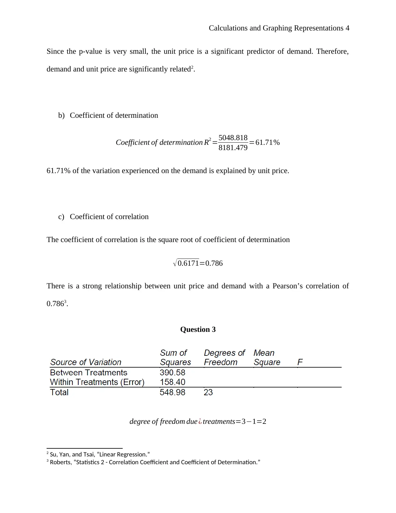
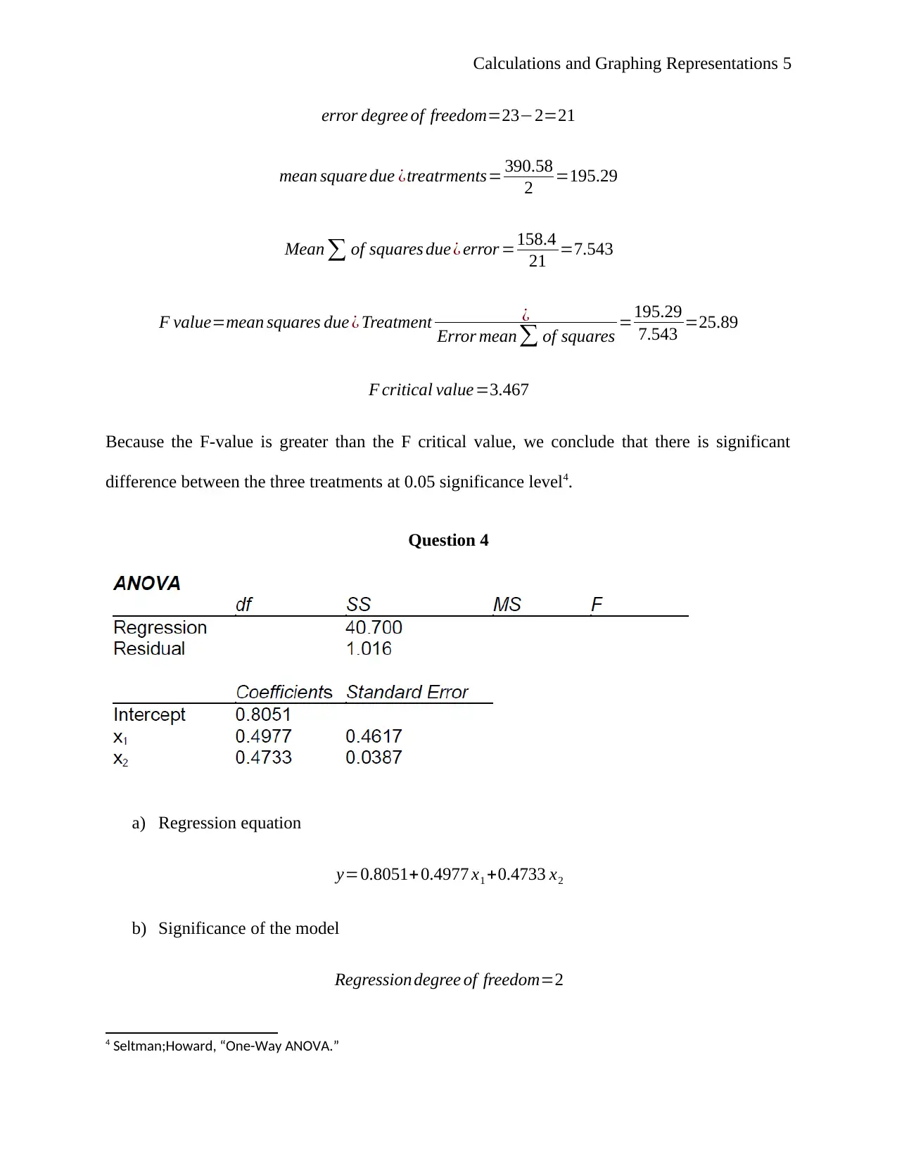
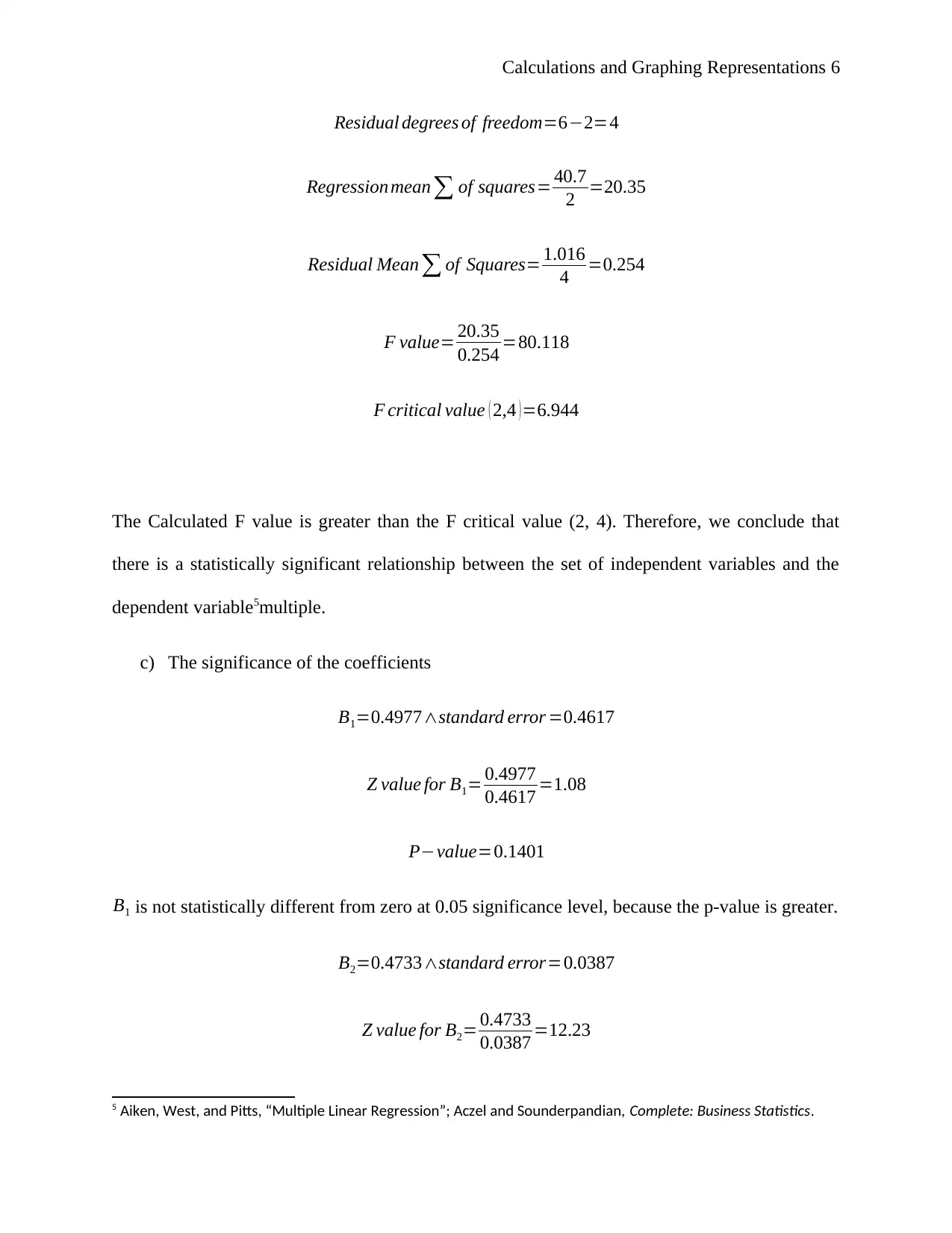
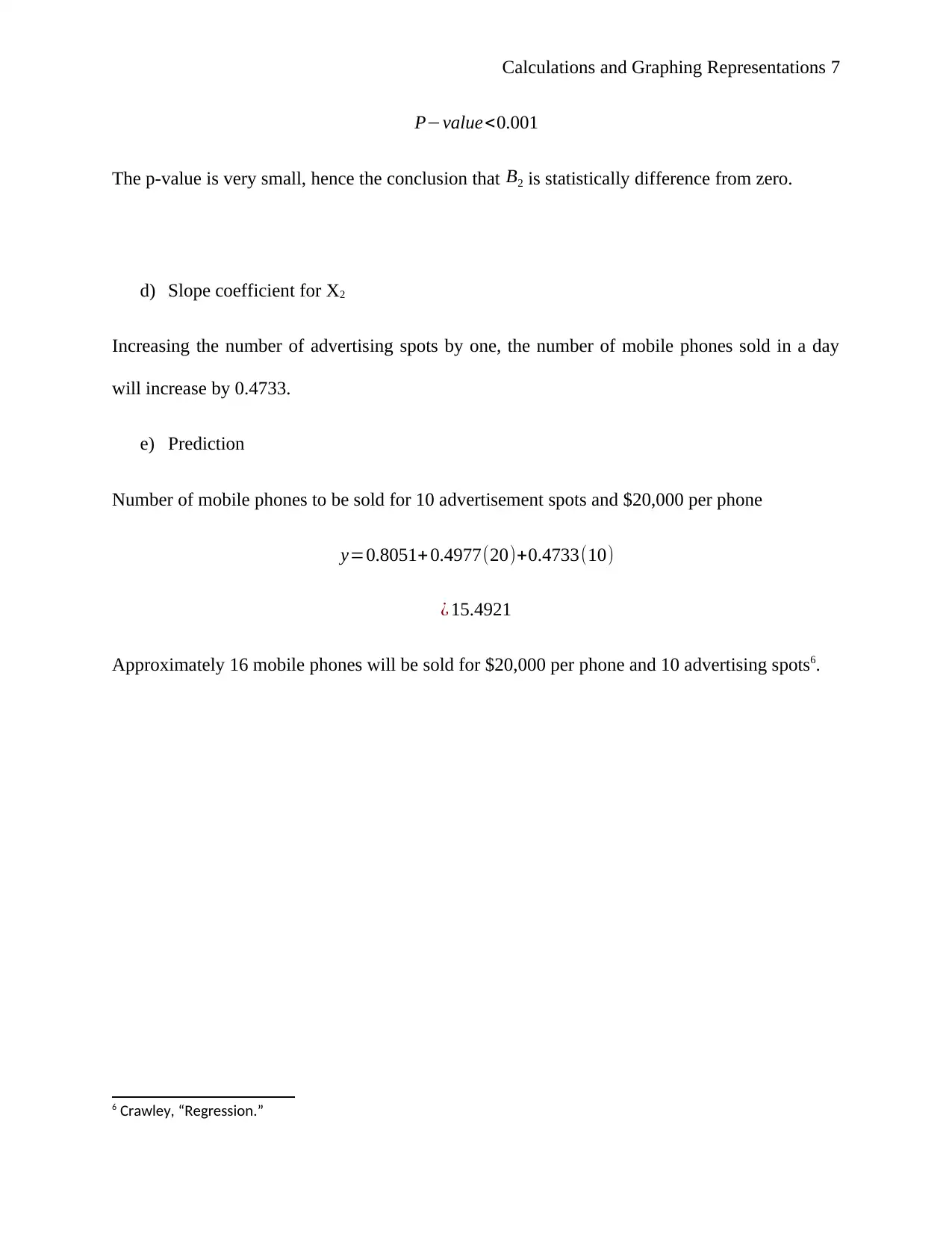
This document presents a solved statistics assignment focusing on calculations and graphing representations. It begins with a frequency distribution table and a histogram visualizing shipping charges, analyzing their distribution, and determining the most appropriate measure of central tendency. The assignment then explores the relationship between demand and unit price, calculating the coefficient of determination and correlation to assess their significance. Further analysis includes an ANOVA test to determine significant differences between treatments and a regression equation to predict mobile phone sales based on advertising spots and phone price. The solution interprets the significance of the model and coefficients, providing predictions and referencing relevant statistical resources.

Calculations and Graphing Representations 1
Calculations and Graphing Representations
Name
Course Number
Date
Faculty Name

Calculations and Graphing Representations 2
Calculations and Graphing Representations
Question 1
a) Frequency distribution
Table 1: Frequency distribution
bin Frequency Relative Frequency Percentage Cumulative Frequency
170 8 0.16 16% 16%
220 15 0.3 30% 46%
270 12 0.24 24% 70%
320 4 0.08 8% 78%
370 5 0.1 10% 88%
420 2 0.04 4% 92%
470 2 0.04 4% 96%
520 2 0.04 4% 100%
b) Histogram of Shipping Charges showing percentages
170 220 270 320 370 420 470 520
0%
5%
10%
15%
20%
25%
30%
35%
Histogram of Shipping Charges
Figure 1: Histogram showing percentages

Calculations and Graphing Representations 3
Shipping charges are highly skewed to the right, showing that there is the extreme value of the
charges. 30% of the values selected are between 170 and 220, 24% between 220 and 270 and
16% between 120 and 170. More than 50% of the values are between 120 and 270 and the
maximum value is 490. Therefore, data on shipping charges are not approximately normal1.
c) The most appropriate measure of central tendency
The median statistic will be the best measure of central tendency because it is not much affected
by extreme values.
Question 2: Demand and Unit price
a) Is demand and Unit Price related?
Demand is the response variable and unit price is the predictor
z statistic= coefficient
standard error
−2.137
0.248 =−8.167
p−value<0.001
1 Aczel and Sounderpandian, Complete: Business Statistics.

Calculations and Graphing Representations 4
Since the p-value is very small, the unit price is a significant predictor of demand. Therefore,
demand and unit price are significantly related2.
b) Coefficient of determination
Coefficient of determination R2 =5048.818
8181.479 =61.71%
61.71% of the variation experienced on the demand is explained by unit price.
c) Coefficient of correlation
The coefficient of correlation is the square root of coefficient of determination
√0.6171=0.786
There is a strong relationship between unit price and demand with a Pearson’s correlation of
0.7863.
Question 3
degree of freedom due ¿ treatments=3−1=2
2 Su, Yan, and Tsai, “Linear Regression.”
3 Roberts, “Statistics 2 - Correlation Coefficient and Coefficient of Determination.”

Calculations and Graphing Representations 5
error degree of freedom=23−2=21
mean square due ¿treatrments= 390.58
2 =195.29
Mean ∑ of squares due ¿ error =158.4
21 =7.543
F value=mean squares due ¿ Treatment ¿
Error mean∑ of squares =195.29
7.543 =25.89
F critical value=3.467
Because the F-value is greater than the F critical value, we conclude that there is significant
difference between the three treatments at 0.05 significance level4.
Question 4
a) Regression equation
y=0.8051+ 0.4977 x1 +0.4733 x2
b) Significance of the model
Regression degree of freedom=2
4 Seltman;Howard, “One-Way ANOVA.”

Calculations and Graphing Representations 6
Residual degrees of freedom=6−2=4
Regression mean∑ of squares= 40.7
2 =20.35
Residual Mean ∑ of Squares= 1.016
4 =0.254
F value= 20.35
0.254 =80.118
F critical value ( 2,4 ) =6.944
The Calculated F value is greater than the F critical value (2, 4). Therefore, we conclude that
there is a statistically significant relationship between the set of independent variables and the
dependent variable5multiple.
c) The significance of the coefficients
B1=0.4977∧standard error =0.4617
Z value for B1= 0.4977
0.4617 =1.08
P−value=0.1401
B1 is not statistically different from zero at 0.05 significance level, because the p-value is greater.
B2=0.4733∧standard error=0.0387
Z value for B2= 0.4733
0.0387 =12.23
5 Aiken, West, and Pitts, “Multiple Linear Regression”; Aczel and Sounderpandian, Complete: Business Statistics.

Calculations and Graphing Representations 7
P−value<0.001
The p-value is very small, hence the conclusion that B2 is statistically difference from zero.
d) Slope coefficient for X2
Increasing the number of advertising spots by one, the number of mobile phones sold in a day
will increase by 0.4733.
e) Prediction
Number of mobile phones to be sold for 10 advertisement spots and $20,000 per phone
y=0.8051+0.4977(20)+0.4733(10)
¿ 15.4921
Approximately 16 mobile phones will be sold for $20,000 per phone and 10 advertising spots6.
6 Crawley, “Regression.”

Calculations and Graphing Representations 8
References
Aczel, A. D, and J Sounderpandian. Complete: Business Statistics. ASSOCIATION OF
BUSINESS INFORMATION …, 2008. http://scholar.google.com/scholar?
hl=en&btnG=Search&q=intitle:McGraw-Hill/Irwin+=%3E?#1.
Aiken, L. S., S. G. West, and S. C. Pitts. “Multiple Linear Regression.” Handbook of
Psychology, 2003, 481–507. https://doi.org/10.1051/eas/1466005.
Crawley, Michael J. “Regression.” In The R Book, 449–97, 2012.
https://doi.org/10.1002/9781118448908.ch10.
Roberts, Donna. “Statistics 2 - Correlation Coefficient and Coefficient of Determination.”
MathBits.com, 2013. http://mathbits.com/MathBits/TISection/Statistics2/correlation.htm.
Seltman, Howard. “One-Way ANOVA.” Experimental Design and Analysis, 2017, 171–90.
https://www.jmp.com/content/dam/jmp/documents/en/academic/learning-library/04-one-
way-anova.pdf.
Su, Xiaogang, Xin Yan, and Chih-Ling Tsai. “Linear Regression.” Wiley Interdisciplinary

Calculations and Graphing Representations 9
Reviews: Computational Statistics 4, no. 3 (2012): 275–94.
https://doi.org/10.1002/wics.1198.