CAM625 Statistics: Problem Analysis, Regression Results & Models
VerifiedAdded on 2023/03/30
|9
|2119
|84
Homework Assignment
AI Summary
This assignment solution covers statistical analysis, focusing on problem analysis and regression techniques. It includes t-tests and chi-square tests to assess the significance of various factors, such as mother's age, race, and BMI, on birth outcomes. Simple and multiple regression models are used to analyze the relationship between variables like gestation length and overweight status, mother's age, and race. Additionally, logistic regression models are employed to investigate the factors influencing parity. The analysis reveals insights into the impact of various variables on gestation length and parity, providing a comprehensive overview of the statistical findings. Desklib offers more solved assignments and past papers for students.
Problem Analysis and Statistics
Student Name:
Instructor Name:
Course Number:
31 May 2019
Student Name:
Instructor Name:
Course Number:
31 May 2019
Paraphrase This Document
Need a fresh take? Get an instant paraphrase of this document with our AI Paraphraser
Task 1:
Continuous variables
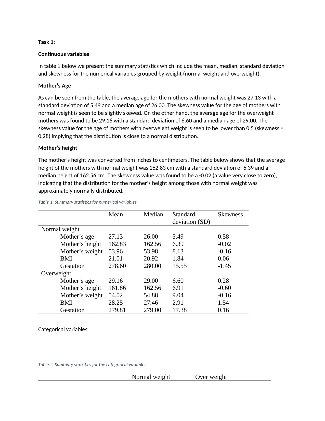
In table 1 below we present the summary statistics which include the mean, median, standard deviation
and skewness for the numerical variables grouped by weight (normal weight and overweight).
Mother’s Age
As can be seen from the table, the average age for the mothers with normal weight was 27.13 with a
standard deviation of 5.49 and a median age of 26.00. The skewness value for the age of mothers with
normal weight is seen to be slightly skewed. On the other hand, the average age for the overweight
mothers was found to be 29.16 with a standard deviation of 6.60 and a median age of 29.00. The
skewness value for the age of mothers with overweight weight is seen to be lower than 0.5 (skewness =
0.28) implying that the distribution is close to a normal distribution.
Mother’s height
The mother’s height was converted from inches to centimeters. The table below shows that the average
height of the mothers with normal weight was 162.83 cm with a standard deviation of 6.39 and a
median height of 162.56 cm. The skewness value was found to be a -0.02 (a value very close to zero),
indicating that the distribution for the mother’s height among those with normal weight was
approximately normally distributed.
Table 1: Summary statistics for numerical variables
Mean Median Standard
deviation (SD)
Skewness
Normal weight
Mother’s age 27.13 26.00 5.49 0.58
Mother’s height 162.83 162.56 6.39 -0.02
Mother’s weight 53.96 53.98 8.13 -0.16
BMI 21.01 20.92 1.84 0.06
Gestation 278.60 280.00 15.55 -1.45
Overweight
Mother’s age 29.16 29.00 6.60 0.28
Mother’s height 161.86 162.56 6.91 -0.60
Mother’s weight 54.02 54.88 9.04 -0.16
BMI 28.25 27.46 2.91 1.54
Gestation 279.81 279.00 17.38 0.16
Categorical variables
Table 2: Summary statistics for the categorical variables
Normal weight Over weight
Continuous variables
In table 1 below we present the summary statistics which include the mean, median, standard deviation
and skewness for the numerical variables grouped by weight (normal weight and overweight).
Mother’s Age
As can be seen from the table, the average age for the mothers with normal weight was 27.13 with a
standard deviation of 5.49 and a median age of 26.00. The skewness value for the age of mothers with
normal weight is seen to be slightly skewed. On the other hand, the average age for the overweight
mothers was found to be 29.16 with a standard deviation of 6.60 and a median age of 29.00. The
skewness value for the age of mothers with overweight weight is seen to be lower than 0.5 (skewness =
0.28) implying that the distribution is close to a normal distribution.
Mother’s height
The mother’s height was converted from inches to centimeters. The table below shows that the average
height of the mothers with normal weight was 162.83 cm with a standard deviation of 6.39 and a
median height of 162.56 cm. The skewness value was found to be a -0.02 (a value very close to zero),
indicating that the distribution for the mother’s height among those with normal weight was
approximately normally distributed.
Table 1: Summary statistics for numerical variables
Mean Median Standard
deviation (SD)
Skewness
Normal weight
Mother’s age 27.13 26.00 5.49 0.58
Mother’s height 162.83 162.56 6.39 -0.02
Mother’s weight 53.96 53.98 8.13 -0.16
BMI 21.01 20.92 1.84 0.06
Gestation 278.60 280.00 15.55 -1.45
Overweight
Mother’s age 29.16 29.00 6.60 0.28
Mother’s height 161.86 162.56 6.91 -0.60
Mother’s weight 54.02 54.88 9.04 -0.16
BMI 28.25 27.46 2.91 1.54
Gestation 279.81 279.00 17.38 0.16
Categorical variables
Table 2: Summary statistics for the categorical variables
Normal weight Over weight
Frequency
(n)
Percent
(%)
Frequency (n) Percent
(%)
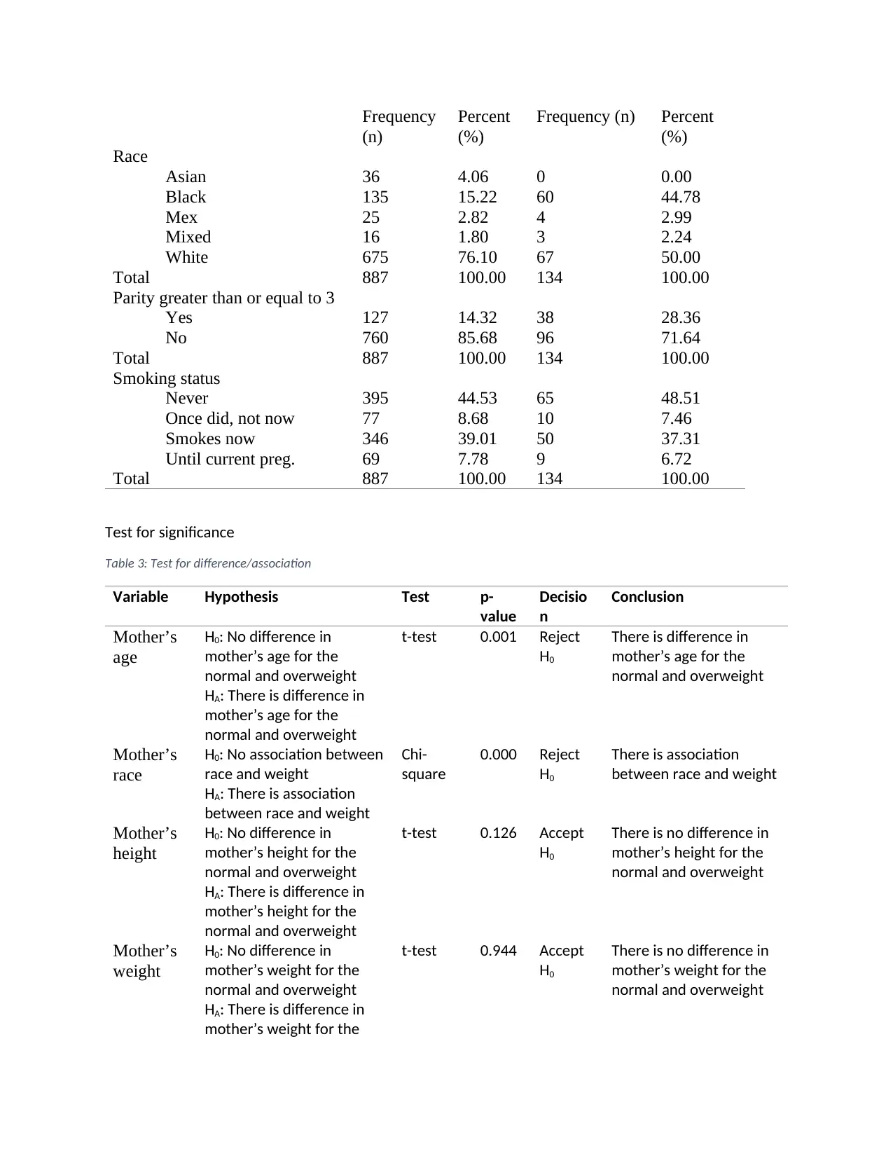
Race
Asian 36 4.06 0 0.00
Black 135 15.22 60 44.78
Mex 25 2.82 4 2.99
Mixed 16 1.80 3 2.24
White 675 76.10 67 50.00
Total 887 100.00 134 100.00
Parity greater than or equal to 3
Yes 127 14.32 38 28.36
No 760 85.68 96 71.64
Total 887 100.00 134 100.00
Smoking status
Never 395 44.53 65 48.51
Once did, not now 77 8.68 10 7.46
Smokes now 346 39.01 50 37.31
Until current preg. 69 7.78 9 6.72
Total 887 100.00 134 100.00
Test for significance
Table 3: Test for difference/association
Variable Hypothesis Test p-
value
Decisio
n
Conclusion
Mother’s
age
H0: No difference in
mother’s age for the
normal and overweight
HA: There is difference in
mother’s age for the
normal and overweight
t-test 0.001 Reject
H0
There is difference in
mother’s age for the
normal and overweight
Mother’s
race
H0: No association between
race and weight
HA: There is association
between race and weight
Chi-
square
0.000 Reject
H0
There is association
between race and weight
Mother’s
height
H0: No difference in
mother’s height for the
normal and overweight
HA: There is difference in
mother’s height for the
normal and overweight
t-test 0.126 Accept
H0
There is no difference in
mother’s height for the
normal and overweight
Mother’s
weight
H0: No difference in
mother’s weight for the
normal and overweight
HA: There is difference in
mother’s weight for the
t-test 0.944 Accept
H0
There is no difference in
mother’s weight for the
normal and overweight
(n)
Percent
(%)
Frequency (n) Percent
(%)
Race
Asian 36 4.06 0 0.00
Black 135 15.22 60 44.78
Mex 25 2.82 4 2.99
Mixed 16 1.80 3 2.24
White 675 76.10 67 50.00
Total 887 100.00 134 100.00
Parity greater than or equal to 3
Yes 127 14.32 38 28.36
No 760 85.68 96 71.64
Total 887 100.00 134 100.00
Smoking status
Never 395 44.53 65 48.51
Once did, not now 77 8.68 10 7.46
Smokes now 346 39.01 50 37.31
Until current preg. 69 7.78 9 6.72
Total 887 100.00 134 100.00
Test for significance
Table 3: Test for difference/association
Variable Hypothesis Test p-
value
Decisio
n
Conclusion
Mother’s
age
H0: No difference in
mother’s age for the
normal and overweight
HA: There is difference in
mother’s age for the
normal and overweight
t-test 0.001 Reject
H0
There is difference in
mother’s age for the
normal and overweight
Mother’s
race
H0: No association between
race and weight
HA: There is association
between race and weight
Chi-
square
0.000 Reject
H0
There is association
between race and weight
Mother’s
height
H0: No difference in
mother’s height for the
normal and overweight
HA: There is difference in
mother’s height for the
normal and overweight
t-test 0.126 Accept
H0
There is no difference in
mother’s height for the
normal and overweight
Mother’s
weight
H0: No difference in
mother’s weight for the
normal and overweight
HA: There is difference in
mother’s weight for the
t-test 0.944 Accept
H0
There is no difference in
mother’s weight for the
normal and overweight
⊘ This is a preview!⊘
Do you want full access?
Subscribe today to unlock all pages.
Trusted by 1+ million students worldwide
normal and overweight
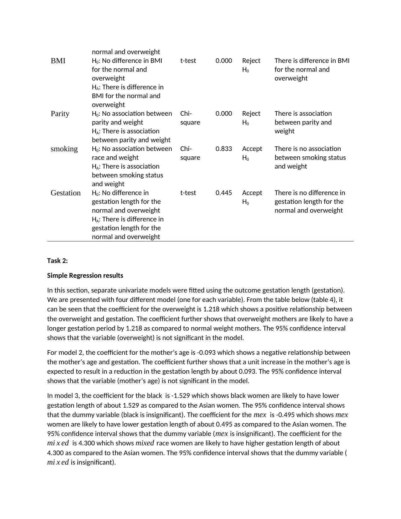
BMI H0: No difference in BMI
for the normal and
overweight
HA: There is difference in
BMI for the normal and
overweight
t-test 0.000 Reject
H0
There is difference in BMI
for the normal and
overweight
Parity H0: No association between
parity and weight
HA: There is association
between parity and weight
Chi-
square
0.000 Reject
H0
There is association
between parity and
weight
smoking H0: No association between
race and weight
HA: There is association
between smoking status
and weight
Chi-
square
0.833 Accept
H0
There is no association
between smoking status
and weight
Gestation H0: No difference in
gestation length for the
normal and overweight
HA: There is difference in
gestation length for the
normal and overweight
t-test 0.445 Accept
H0
There is no difference in
gestation length for the
normal and overweight
Task 2:
Simple Regression results
In this section, separate univariate models were fitted using the outcome gestation length (gestation).
We are presented with four different model (one for each variable). From the table below (table 4), it
can be seen that the coefficient for the overweight is 1.218 which shows a positive relationship between
the overweight and gestation. The coefficient further shows that overweight mothers are likely to have a
longer gestation period by 1.218 as compared to normal weight mothers. The 95% confidence interval
shows that the variable (overweight) is not significant in the model.
For model 2, the coefficient for the mother’s age is -0.093 which shows a negative relationship between
the mother’s age and gestation. The coefficient further shows that a unit increase in the mother’s age is
expected to result in a reduction in the gestation length by about 0.093. The 95% confidence interval
shows that the variable (mother’s age) is not significant in the model.
In model 3, the coefficient for the black is -1.529 which shows black women are likely to have lower
gestation length of about 1.529 as compared to the Asian women. The 95% confidence interval shows
that the dummy variable (black is insignificant). The coefficient for the mex is -0.495 which shows mex
women are likely to have lower gestation length of about 0.495 as compared to the Asian women. The
95% confidence interval shows that the dummy variable ( mex is insignificant). The coefficient for the
mi x ed is 4.300 which shows mixed race women are likely to have higher gestation length of about
4.300 as compared to the Asian women. The 95% confidence interval shows that the dummy variable (
mi x ed is insignificant).
Paraphrase This Document
Need a fresh take? Get an instant paraphrase of this document with our AI Paraphraser
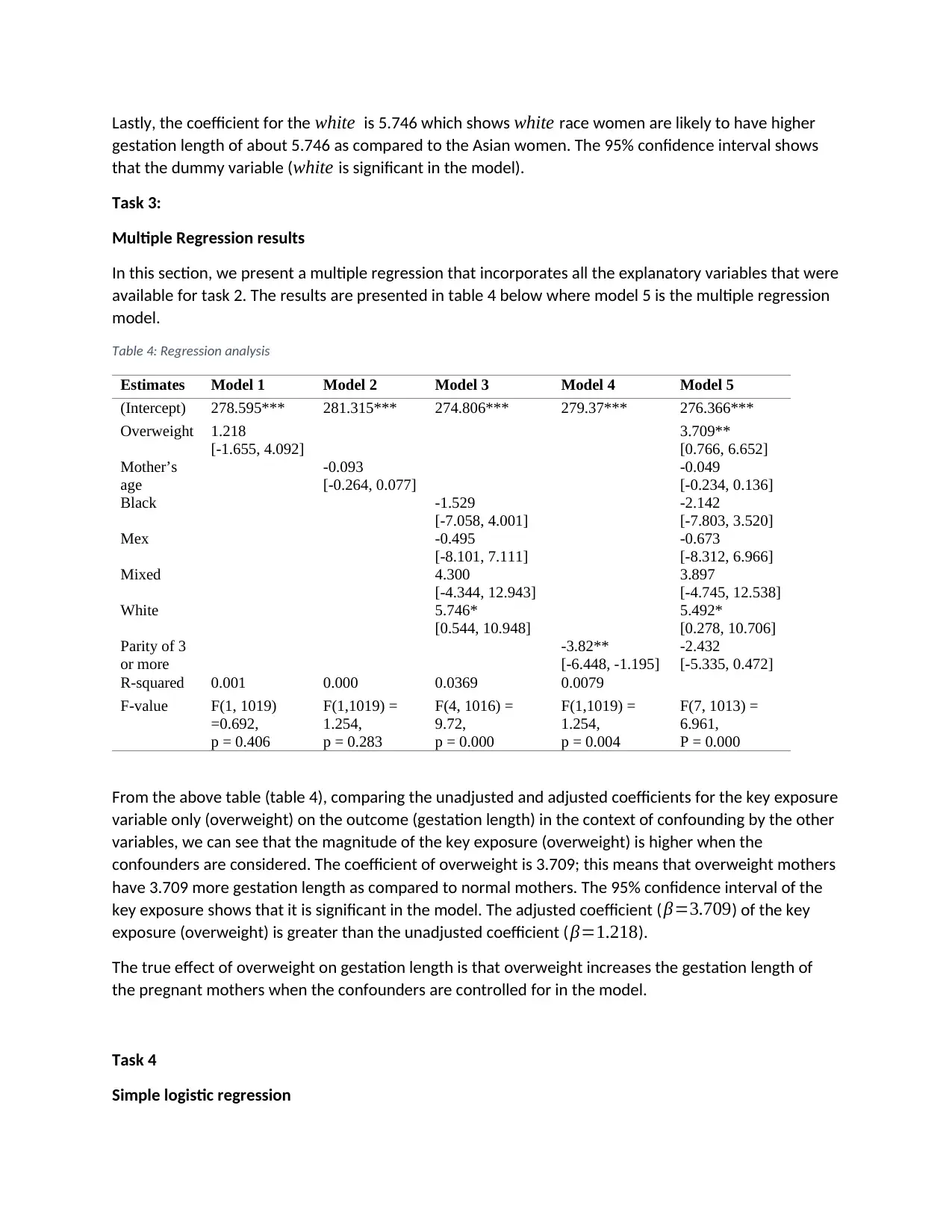
Lastly, the coefficient for the white is 5.746 which shows white race women are likely to have higher
gestation length of about 5.746 as compared to the Asian women. The 95% confidence interval shows
that the dummy variable (white is significant in the model).
Task 3:
Multiple Regression results
In this section, we present a multiple regression that incorporates all the explanatory variables that were
available for task 2. The results are presented in table 4 below where model 5 is the multiple regression
model.
Table 4: Regression analysis
Estimates Model 1 Model 2 Model 3 Model 4 Model 5
(Intercept) 278.595*** 281.315*** 274.806*** 279.37*** 276.366***
Overweight 1.218
[-1.655, 4.092]
3.709**
[0.766, 6.652]
Mother’s
age
-0.093
[-0.264, 0.077]
-0.049
[-0.234, 0.136]
Black -1.529
[-7.058, 4.001]
-2.142
[-7.803, 3.520]
Mex -0.495
[-8.101, 7.111]
-0.673
[-8.312, 6.966]
Mixed 4.300
[-4.344, 12.943]
3.897
[-4.745, 12.538]
White 5.746*
[0.544, 10.948]
5.492*
[0.278, 10.706]
Parity of 3
or more
-3.82**
[-6.448, -1.195]
-2.432
[-5.335, 0.472]
R-squared 0.001 0.000 0.0369 0.0079
F-value F(1, 1019)
=0.692,
p = 0.406
F(1,1019) =
1.254,
p = 0.283
F(4, 1016) =
9.72,
p = 0.000
F(1,1019) =
1.254,
p = 0.004
F(7, 1013) =
6.961,
P = 0.000
From the above table (table 4), comparing the unadjusted and adjusted coefficients for the key exposure
variable only (overweight) on the outcome (gestation length) in the context of confounding by the other
variables, we can see that the magnitude of the key exposure (overweight) is higher when the
confounders are considered. The coefficient of overweight is 3.709; this means that overweight mothers
have 3.709 more gestation length as compared to normal mothers. The 95% confidence interval of the
key exposure shows that it is significant in the model. The adjusted coefficient ( β=3.709) of the key
exposure (overweight) is greater than the unadjusted coefficient ( β=1.218).
The true effect of overweight on gestation length is that overweight increases the gestation length of
the pregnant mothers when the confounders are controlled for in the model.
Task 4
Simple logistic regression
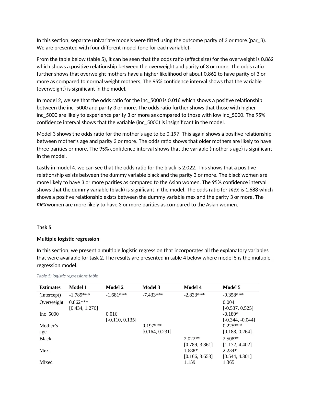
In this section, separate univariate models were fitted using the outcome parity of 3 or more (par_3).
We are presented with four different model (one for each variable).
From the table below (table 5), it can be seen that the odds ratio (effect size) for the overweight is 0.862
which shows a positive relationship between the overweight and parity of 3 or more. The odds ratio
further shows that overweight mothers have a higher likelihood of about 0.862 to have parity of 3 or
more as compared to normal weight mothers. The 95% confidence interval shows that the variable
(overweight) is significant in the model.
In model 2, we see that the odds ratio for the inc_5000 is 0.016 which shows a positive relationship
between the inc_5000 and parity 3 or more. The odds ratio further shows that those with higher
inc_5000 are likely to experience parity 3 or more as compared to those with low inc_5000. The 95%
confidence interval shows that the variable (inc_5000) is insignificant in the model.
Model 3 shows the odds ratio for the mother’s age to be 0.197. This again shows a positive relationship
between mother’s age and parity 3 or more. The odds ratio shows that older mothers are likely to have
three parities or more. The 95% confidence interval shows that the variable (mother’s age) is significant
in the model.
Lastly in model 4, we can see that the odds ratio for the black is 2.022. This shows that a positive
relationship exists between the dummy variable black and the parity 3 or more. The black women are
more likely to have 3 or more parities as compared to the Asian women. The 95% confidence interval
shows that the dummy variable (black) is significant in the model. The odds ratio for mex is 1.688 which
shows a positive relationship exists between the dummy variable mex and the parity 3 or more. The
mexwomen are more likely to have 3 or more parities as compared to the Asian women.
Task 5
Multiple logistic regression
In this section, we present a multiple logistic regression that incorporates all the explanatory variables
that were available for task 2. The results are presented in table 4 below where model 5 is the multiple
regression model.
Table 5: logistic regressions table
Estimates Model 1 Model 2 Model 3 Model 4 Model 5
(Intercept) -1.789*** -1.681*** -7.433*** -2.833*** -9.358***
Overweight 0.862***
[0.434, 1.276]
0.004
[-0.537, 0.525]
Inc_5000 0.016
[-0.110, 0.135]
-0.189*
[-0.344, -0.044]
Mother’s
age
0.197***
[0.164, 0.231]
0.225***
[0.188, 0.264]
Black 2.022**
[0.789, 3.861]
2.508**
[1.172, 4.402]
Mex 1.688*
[0.166, 3.653]
2.234*
[0.544, 4.301]
Mixed 1.159 1.365
⊘ This is a preview!⊘
Do you want full access?
Subscribe today to unlock all pages.
Trusted by 1+ million students worldwide
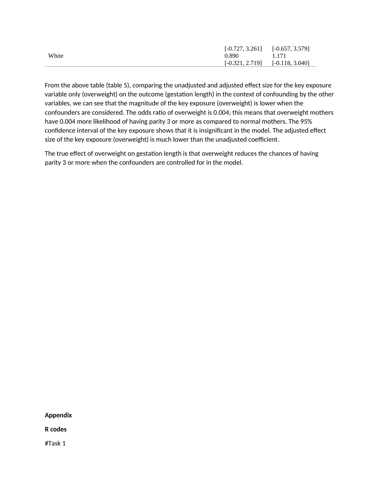
[-0.727, 3.261] [-0.657, 3.579]
White 0.890
[-0.321, 2.719]
1.171
[-0.118, 3.040]
From the above table (table 5), comparing the unadjusted and adjusted effect size for the key exposure
variable only (overweight) on the outcome (gestation length) in the context of confounding by the other
variables, we can see that the magnitude of the key exposure (overweight) is lower when the
confounders are considered. The odds ratio of overweight is 0.004; this means that overweight mothers
have 0.004 more likelihood of having parity 3 or more as compared to normal mothers. The 95%
confidence interval of the key exposure shows that it is insignificant in the model. The adjusted effect
size of the key exposure (overweight) is much lower than the unadjusted coefficient.
The true effect of overweight on gestation length is that overweight reduces the chances of having
parity 3 or more when the confounders are controlled for in the model.
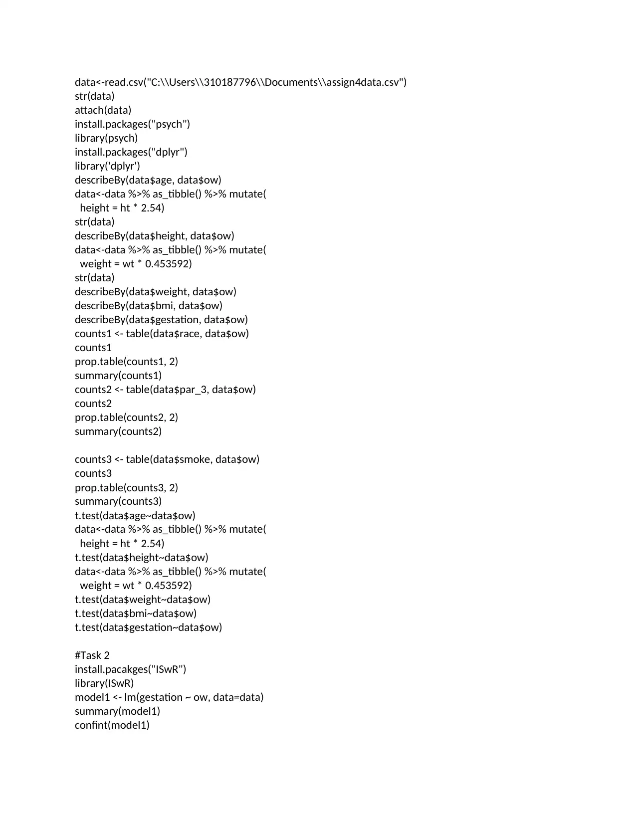
Appendix
R codes
#Task 1
White 0.890
[-0.321, 2.719]
1.171
[-0.118, 3.040]
From the above table (table 5), comparing the unadjusted and adjusted effect size for the key exposure
variable only (overweight) on the outcome (gestation length) in the context of confounding by the other
variables, we can see that the magnitude of the key exposure (overweight) is lower when the
confounders are considered. The odds ratio of overweight is 0.004; this means that overweight mothers
have 0.004 more likelihood of having parity 3 or more as compared to normal mothers. The 95%
confidence interval of the key exposure shows that it is insignificant in the model. The adjusted effect
size of the key exposure (overweight) is much lower than the unadjusted coefficient.
The true effect of overweight on gestation length is that overweight reduces the chances of having
parity 3 or more when the confounders are controlled for in the model.
Appendix
R codes
#Task 1
Paraphrase This Document
Need a fresh take? Get an instant paraphrase of this document with our AI Paraphraser
data<-read.csv("C:\\Users\\310187796\\Documents\\assign4data.csv")
str(data)
attach(data)
install.packages("psych")
library(psych)
install.packages("dplyr")
library('dplyr')
describeBy(data$age, data$ow)
data<-data %>% as_tibble() %>% mutate(
height = ht * 2.54)
str(data)
describeBy(data$height, data$ow)
data<-data %>% as_tibble() %>% mutate(
weight = wt * 0.453592)
str(data)
describeBy(data$weight, data$ow)
describeBy(data$bmi, data$ow)
describeBy(data$gestation, data$ow)
counts1 <- table(data$race, data$ow)
counts1
prop.table(counts1, 2)
summary(counts1)
counts2 <- table(data$par_3, data$ow)
counts2
prop.table(counts2, 2)
summary(counts2)
counts3 <- table(data$smoke, data$ow)
counts3
prop.table(counts3, 2)
summary(counts3)
t.test(data$age~data$ow)
data<-data %>% as_tibble() %>% mutate(
height = ht * 2.54)
t.test(data$height~data$ow)
data<-data %>% as_tibble() %>% mutate(
weight = wt * 0.453592)
t.test(data$weight~data$ow)
t.test(data$bmi~data$ow)
t.test(data$gestation~data$ow)
#Task 2
install.pacakges("ISwR")
library(ISwR)
model1 <- lm(gestation ~ ow, data=data)
summary(model1)
confint(model1)
str(data)
attach(data)
install.packages("psych")
library(psych)
install.packages("dplyr")
library('dplyr')
describeBy(data$age, data$ow)
data<-data %>% as_tibble() %>% mutate(
height = ht * 2.54)
str(data)
describeBy(data$height, data$ow)
data<-data %>% as_tibble() %>% mutate(
weight = wt * 0.453592)
str(data)
describeBy(data$weight, data$ow)
describeBy(data$bmi, data$ow)
describeBy(data$gestation, data$ow)
counts1 <- table(data$race, data$ow)
counts1
prop.table(counts1, 2)
summary(counts1)
counts2 <- table(data$par_3, data$ow)
counts2
prop.table(counts2, 2)
summary(counts2)
counts3 <- table(data$smoke, data$ow)
counts3
prop.table(counts3, 2)
summary(counts3)
t.test(data$age~data$ow)
data<-data %>% as_tibble() %>% mutate(
height = ht * 2.54)
t.test(data$height~data$ow)
data<-data %>% as_tibble() %>% mutate(
weight = wt * 0.453592)
t.test(data$weight~data$ow)
t.test(data$bmi~data$ow)
t.test(data$gestation~data$ow)
#Task 2
install.pacakges("ISwR")
library(ISwR)
model1 <- lm(gestation ~ ow, data=data)
summary(model1)
confint(model1)

model2 <- lm(gestation ~ age, data=data)
summary(model2)
confint(model2)
model3 <- lm(gestation ~ race, data=data)
summary(model3)
confint(model3)
model4 <- lm(gestation ~ par_3, data=data)
summary(model4)
confint(model4)
#Task 3
model5 <- lm(gestation ~ ow+age+race+par_3, data=data)
summary(model5)
confint(model5)
#task 4
model6 <- glm(formula=par_3 ~ ow, family = "binomial", data=data)
summary(model6)
confint(model6)
model7 <- glm(formula=par_3 ~ inc_5000, family = "binomial", data=data)
summary(model7)
confint(model7)
model8 <- glm(formula=par_3 ~ age, family = "binomial", data=data)
summary(model8)
confint(model8)
model9 <- glm(formula=par_3 ~ race, family = "binomial", data=data)
summary(model9)
confint(model9)
#task 5
model10 <- glm(formula=par_3 ~ow+inc_5000+age+race, family = "binomial", data=data)
summary(model10)
confint(model10)
⊘ This is a preview!⊘
Do you want full access?
Subscribe today to unlock all pages.
Trusted by 1+ million students worldwide
1 out of 9
Your All-in-One AI-Powered Toolkit for Academic Success.
+13062052269
info@desklib.com
Available 24*7 on WhatsApp / Email
![[object Object]](/_next/static/media/star-bottom.7253800d.svg)
Unlock your academic potential
Copyright © 2020–2026 A2Z Services. All Rights Reserved. Developed and managed by ZUCOL.