An Analysis of the Capital Asset Pricing Model (CAPM)
VerifiedAdded on 2021/05/27
|15
|3664
|89
Report
AI Summary
This report provides a comprehensive analysis of the Capital Asset Pricing Model (CAPM), a financial model used to evaluate the relationship between expected returns and risks associated with investments. The report defines CAPM, explains its formula, and illustrates its application with a practical calculation example. It delves into the model's key assumptions, such as diversified portfolios and a perfect capital market, while also acknowledging their limitations in the real world. The report critically examines the criticisms and limitations of CAPM, including its unrealistic assumptions and statistical deficiencies. Furthermore, it explores alternative models like the Intertemporal Capital Asset Pricing Model (ICAPM) and the Consumption Capital Asset Pricing Model (CCAPM) to address CAPM's shortcomings. The report also discusses other asset pricing models, such as Arbitrage Pricing Theory (APT) and the Three-Factor Model, offering a broader perspective on investment analysis. Overall, the report offers valuable insights into the CAPM model, its applications, and its place in the financial world.

CAPM 1
Capital asset pricing model (CAPM)
by Student Name
The Name of the Class (Course)
Professor
The Name of the University
The City & State
Date
Capital asset pricing model (CAPM)
by Student Name
The Name of the Class (Course)
Professor
The Name of the University
The City & State
Date
Paraphrase This Document
Need a fresh take? Get an instant paraphrase of this document with our AI Paraphraser
CAPM 2
Capital asset pricing model (CAPM)
Introduction
The Capital asset pricing model (CAPM) is a beneficial model, and it is used widely in the
industry even though it is based on extreme assumptions. In line with this statement, this
paper seeks to investigate on the issues surrounding CAPM as a financial/ investment concept
heavily relied upon by the investors in the economic and investment markets. Specifically,
the study seeks to address the specific issues surrounding CAPM such as its definition, key
assumptions, criticisms and limitations, other alternative financial models that can be used in
place of CAPM and the application of CAPM.
Description of CAPM
The Capital Asset Pricing Model (CAPM) is a financial/ investment model used by to
evaluate the relationship between expected returns and risks associated with an investment. In
the real world, investors take up investment risks with a hope of higher returns (Fama &
French, 2004, p. 27). The CAPM model demonstrates that the expected return should be
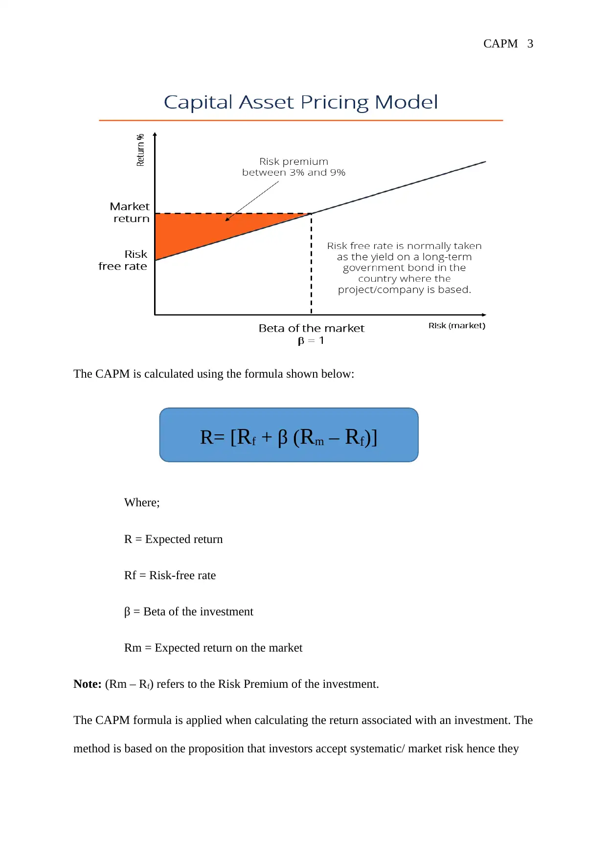
equivalent to the risk premium plus risk-free returns based of the beta of a given investment.
The linear relationship between the expected return and its systematic risk is presented as
below;
Capital asset pricing model (CAPM)
Introduction
The Capital asset pricing model (CAPM) is a beneficial model, and it is used widely in the
industry even though it is based on extreme assumptions. In line with this statement, this
paper seeks to investigate on the issues surrounding CAPM as a financial/ investment concept
heavily relied upon by the investors in the economic and investment markets. Specifically,
the study seeks to address the specific issues surrounding CAPM such as its definition, key
assumptions, criticisms and limitations, other alternative financial models that can be used in
place of CAPM and the application of CAPM.
Description of CAPM
The Capital Asset Pricing Model (CAPM) is a financial/ investment model used by to
evaluate the relationship between expected returns and risks associated with an investment. In
the real world, investors take up investment risks with a hope of higher returns (Fama &
French, 2004, p. 27). The CAPM model demonstrates that the expected return should be
equivalent to the risk premium plus risk-free returns based of the beta of a given investment.
The linear relationship between the expected return and its systematic risk is presented as
below;
CAPM 3
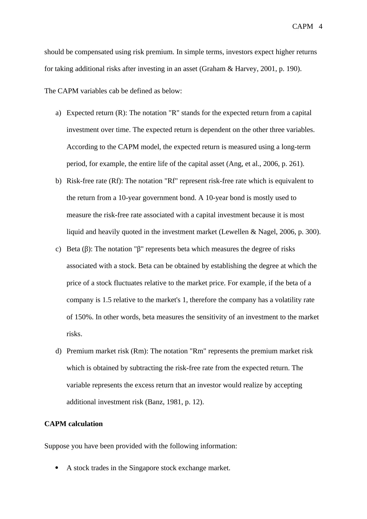
The CAPM is calculated using the formula shown below:
Where;
R = Expected return
Rf = Risk-free rate
β = Beta of the investment
Rm = Expected return on the market
Note: (Rm – Rf) refers to the Risk Premium of the investment.
The CAPM formula is applied when calculating the return associated with an investment. The
method is based on the proposition that investors accept systematic/ market risk hence they
R= [Rf + β (Rm – Rf)]
⊘ This is a preview!⊘
Do you want full access?
Subscribe today to unlock all pages.
Trusted by 1+ million students worldwide
CAPM 4
should be compensated using risk premium. In simple terms, investors expect higher returns
for taking additional risks after investing in an asset (Graham & Harvey, 2001, p. 190).
The CAPM variables cab be defined as below:
a) Expected return (R): The notation "R" stands for the expected return from a capital
investment over time. The expected return is dependent on the other three variables.
According to the CAPM model, the expected return is measured using a long-term
period, for example, the entire life of the capital asset (Ang, et al., 2006, p. 261).
b) Risk-free rate (Rf): The notation "Rf" represent risk-free rate which is equivalent to
the return from a 10-year government bond. A 10-year bond is mostly used to
measure the risk-free rate associated with a capital investment because it is most
liquid and heavily quoted in the investment market (Lewellen & Nagel, 2006, p. 300).
c) Beta (β): The notation "β" represents beta which measures the degree of risks
associated with a stock. Beta can be obtained by establishing the degree at which the
price of a stock fluctuates relative to the market price. For example, if the beta of a
company is 1.5 relative to the market's 1, therefore the company has a volatility rate
of 150%. In other words, beta measures the sensitivity of an investment to the market
risks.
d) Premium market risk (Rm): The notation "Rm" represents the premium market risk
which is obtained by subtracting the risk-free rate from the expected return. The
variable represents the excess return that an investor would realize by accepting
additional investment risk (Banz, 1981, p. 12).
CAPM calculation
Suppose you have been provided with the following information:
A stock trades in the Singapore stock exchange market.
Paraphrase This Document
Need a fresh take? Get an instant paraphrase of this document with our AI Paraphraser
CAPM 5
Its current yield based on a ten year Singapore bond is 3.5%.
Historically the stock has an annual return of 6.5%.
The stock has a beta of 1.26.
Calculate the expected return on the investment using the CAPM formula.
Expected return = [Risk Free Rate + (Beta x Market Return Premium)]
R= [Rf + β (Rm – Rf)]
R= [Rf + β (Rm – Rf)]
R= 3.5% + [1.26 x 6.5%]
R= 11.69%
Therefore, the expected return on the investment is 11.9%.
CAPM Assumptions
The CAPM model has received criticism from different quarters because of its unrealistic
assumptions. This section discusses the four main assumptions of CAPM and their
applicability in the real world. The premises are:
First, Investors hold diversified portfolios. The assumption states that investors should rely on
systematic risk when choosing an investment portfolio. The unsystematic risk is ignored
because it is diversified (Sharpe, 1964, p. 427).
In the real world, it is impossible for investors to hold an entire market portfolio. However, it
is inexpensive and more manageable for investors to diversify unsystematic risk which offers
an opportunity for an expected return to relying entirely on the systematic risk. Therefore the
assumption is reasonable where investors only focus on acquiring systematic risk for
financial compensation (Kellerhals, 2013, p. 76).
CAPM 6
Second, single-period transaction horizon. CAPM model prefers to apply a standardized
period for different investments for comparability purposes. In other words, returns realized
from a six-month investment cannot be compared to returns realized from a twelve-month
investment. CAPM usually uses a one year as a universally acceptable holding period (Fama
& French, 2006, p. 2172).
In the real world, a single period transaction horizon is reasonable. Although investors hold
investment portfolio for at least one year, the returns are disclosed on an annual basis.
Therefore, using a one year horizon period realistic in the investment market.
Third, investors can borrow and lend at the risk-free rate of return. The assumption was
developed from the portfolio theory which was used to establish the CAPM model as well. In
other words, investors can borrow and lend freely without worrying about additional risk
(Bailey, 2005, p. 132).
However, the assumption cannot hold in the real world. In the investment market, the risk
associated with individual investments is higher compared to the risk associated with the
government investments. Therefore, in the real world, there is no possibility of borrowing and
lending at a risk-free rate. The inability to borrow and lend at a risk-free rate makes the
assumption unrealistic.
Fourth the capital market is perfect. The assumption means that investments in the market are
valued correctly. An ideal market is associated with the following attributes. First, there are
no transaction costs and taxes related to investments. Second, information can be freely
accessed by all investors at the same time. Third, all investors in the market are well informed
about the risk. Fourth, all investors are rational decision-makers and possess the desire to
maximize the return from their securities. And fifth, the market has many sellers and buyers
(Economou, et al., 2017).
⊘ This is a preview!⊘
Do you want full access?
Subscribe today to unlock all pages.
Trusted by 1+ million students worldwide
CAPM 7
The perfect capital market assumption allows the CAPM model to present a relationship
between expected return and systematic risk. Although the assumption work in an idealized
world, it does not give the same results in the real world.
In the real-world capital markets are not perfect. In developed investment markets,
information is not freely available to the investment. Realistically, information is sold to the
highest buyers. Likewise, capital markets are characterized by transaction costs and taxes.
Lastly, the price of securities, as well as the revenues associated with such securities, cannot
be estimated accurately making it challenging to present a relationship between expected
return and systematic risk (Levy, 2012, p. 45).
Overall while some assumptions are unrealistic, some are realistic. Although most of the
assumptions make sense when applied in the idealized world, there is a possibility of
implementing them in the real world to obtain a linear relationship between expected return
and systematic risk (Kothari Et Al., 1995, p. 197).
Critique of CAPM
The CAPM's assumptions make the model unrealistic and difficult to apply in the real world.
The real capital market does not comprise of assumptions. For instance, free capital markets
do not exist; risk-free lending and borrowing is not realistic; different securities have
different taxes; not all investors are rational when it comes to decision making, and the
information is not free. The assumptions have been used as the basis for criticizing the
CAPM model.
According to Roll (1977), the CAPM is incorrect, and the model cannot be tested when the
real market portfolio is unknown. Roll used a proxy market (S&P 500) to justify the problems
associated with the CAPM model. First, when the S&P 500 proved to be efficient, the market
Paraphrase This Document
Need a fresh take? Get an instant paraphrase of this document with our AI Paraphraser
CAPM 8
portfolio was not. And second, there was no explanation for the market portfolio is efficient
when S&P 500 was inefficient.
The attempt by CAPM to measure the relationship between the expected revenue and beta
values as single equity is unrealistic. Market index (S&P 500) comprises of the index of all
securities and not a single entity. A market index should comprise of bonds, foreign assets,
tangible or intangible human capital and property. Unless the market portfolio is known, the
accuracy and efficiency of the CAPM model cannot be ascertained (Fama & French, 1993, p.
34).
According to Jeng (2018, p. 178), CAPM model is affected by the statistical deficiency. By
ignoring risks such as P/E ratio, book-to-market equity value and company size make it
difficult to prove the accuracy of the model.
The findings by Roll (1977) was also supported by Jagannathan and McGrattan (1995). The
study found out that the CAPM model is inappropriate as a result of its assumptions. A real
market should comprise of all factors in the economy. CAPM does not capture intangible
assets like human capital which profoundly influence the performance of an investment in a
capital market.
New directions to resolve challenges
Two models were developed to address the challenges experienced under CAPM. The
models are the Intertemporal Capital Asset Pricing Model (ICAPM) and the Consumption
Capital Asset Pricing Model (CCAPM).
a) Intertemporal Capital Asset Pricing Model (ICAPM)
Merton developed ICAPM in 1973 as an improved version of CAPM. ICPAM takes into
account the time-varying factors. The model assumes that investors take into account the
CAPM 9
current and future risk factors like inflation, unemployment rate and future returns (Riley,
2009).
Considering that investors' appetite for risk varies, the ICAPM model a men variance analysis
to mitigate projected risk from one investor to another. The mean-variance analysis makes it
easier to arrive at a normal distribution of risk over time. Lastly, ICAPM formula comprises
of several beta coefficients representing different hedging portfolios (Berk, 1995, p. 281).
The ICAPM formula is:
Ri = Rf + β*(Rm-Rf) + βj*(Rn – Rf)
Where:
Ri = Expected return
Rf = Risk-free rate
Rm = Return on the market portfolio and
Rn = Expected return on the hedging
β = Measure of systematic risk concerning the market portfolio
βj= Represents the measure of volatility concerning the hedging security
b) Consumption Capital Asset Pricing Model (CCAPM)
Breeden created the CCAPM in 1979 as an improved version of the CAPM model. Unlike
CAPM that uses a market beta, CCAPM uses consumption beta to determine the expected
return premiums over the risk-free rate. According to CCAPM security premiums are
determined by consumption betas. CCAPM is useful because it allows measurement of risks
associated with stock based on the consumption growth. The higher the consumption beta,
the higher the expected return on a security.
⊘ This is a preview!⊘
Do you want full access?
Subscribe today to unlock all pages.
Trusted by 1+ million students worldwide
CAPM 10
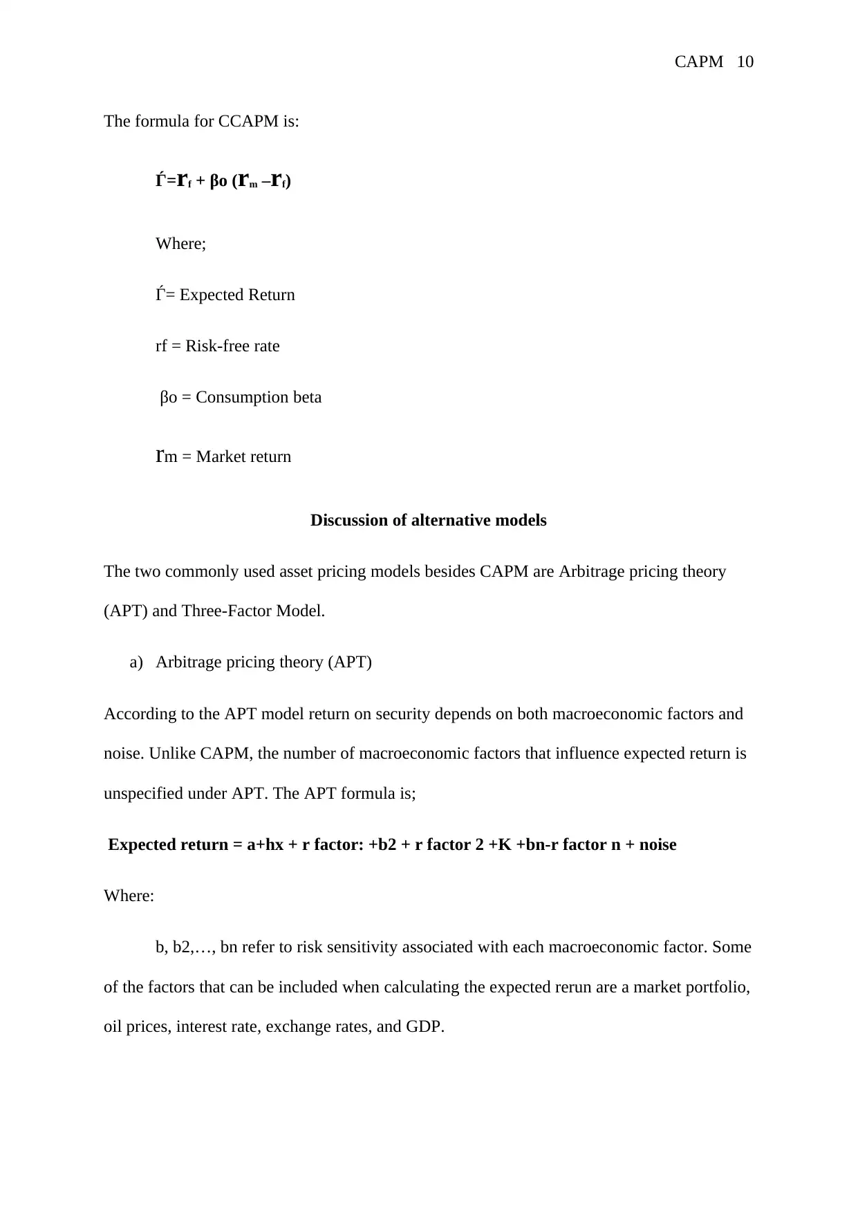
The formula for CCAPM is:
Ѓ=rf + βo (rm –rf)
Where;
Ѓ= Expected Return
rf = Risk-free rate
βo = Consumption beta
rm = Market return
Discussion of alternative models
The two commonly used asset pricing models besides CAPM are Arbitrage pricing theory
(APT) and Three-Factor Model.
a) Arbitrage pricing theory (APT)
According to the APT model return on security depends on both macroeconomic factors and
noise. Unlike CAPM, the number of macroeconomic factors that influence expected return is
unspecified under APT. The APT formula is;
Expected return = a+hx + r factor: +b2 + r factor 2 +K +bn-r factor n + noise
Where:
b, b2,…, bn refer to risk sensitivity associated with each macroeconomic factor. Some
of the factors that can be included when calculating the expected rerun are a market portfolio,
oil prices, interest rate, exchange rates, and GDP.
Paraphrase This Document
Need a fresh take? Get an instant paraphrase of this document with our AI Paraphraser
CAPM 11
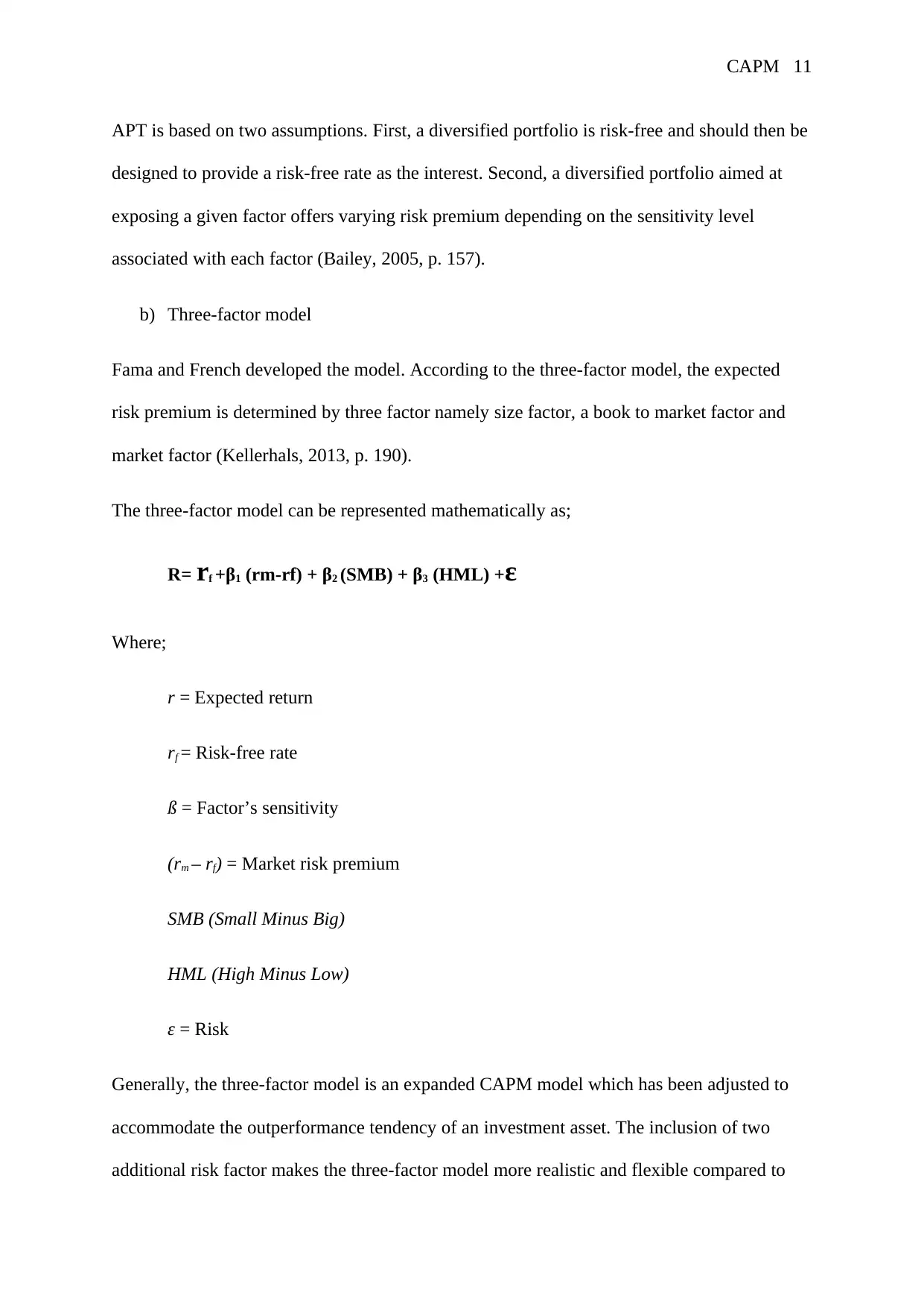
APT is based on two assumptions. First, a diversified portfolio is risk-free and should then be
designed to provide a risk-free rate as the interest. Second, a diversified portfolio aimed at
exposing a given factor offers varying risk premium depending on the sensitivity level
associated with each factor (Bailey, 2005, p. 157).
b) Three-factor model
Fama and French developed the model. According to the three-factor model, the expected
risk premium is determined by three factor namely size factor, a book to market factor and
market factor (Kellerhals, 2013, p. 190).
The three-factor model can be represented mathematically as;
R= rf +β1 (rm-rf) + β2 (SMB) + β3 (HML) +ε
Where;
r = Expected return
rf = Risk-free rate
ß = Factor’s sensitivity
(rm – rf) = Market risk premium
SMB (Small Minus Big)
HML (High Minus Low)
ε = Risk
Generally, the three-factor model is an expanded CAPM model which has been adjusted to
accommodate the outperformance tendency of an investment asset. The inclusion of two
additional risk factor makes the three-factor model more realistic and flexible compared to
CAPM 12
CAPM. Currently, the three-factor model has been expanded further to include the four-factor
model and the five-factor model.
Uses of CAPM
CAPM has several applications; some of the common uses have been mentioned below:
a) Investment Comparison: CAPM is used by investors to compare and contrast different
securities. For instance, securities such as equities, bonds and stocks can be analyzed
using CAPM to help in generating an investment portfolio that maximizes expected
return and reduced associated risk (Banz, 1981, p. 18).
b) Pricing of Assets and Portfolio: CAPM is used to calculate the value of a portfolio or
an asset as a way to determine its worth. Investors use CAPM to determine whether or
not an asset or portfolio is likely to uphold its value in the long run.
c) Calculate the Intrinsic value of an asset: Financial analysts and investors use CAPM
to determine the adjacent between the book and market value of a security. An
investor should only invest in security when it is trading below its intrinsic value.
d) Calculating NPV: CAPM diversifies all the risks associated with an asset. Therefore,
it can be relied upon when calculating NPV for an investment (Levy, 2012, p. 57).
Conclusions
CAPM model as a financial/ investment concept is heavily relied upon by the investors when
making investment decisions. However, the model has been criticized by many because of its
overreliance on several assumptions. Critics argue that without the assumptions (most of
which are unrealistic) the CAPM model cannot hold. The study found out that while some
assumptions are unrealistic, some are realistic. Even though most of the assumptions make
sense when applied in the idealized world, there is a possibility of applying them in the real
world to obtain a linear relationship between expected return and systematic risk.
⊘ This is a preview!⊘
Do you want full access?
Subscribe today to unlock all pages.
Trusted by 1+ million students worldwide
1 out of 15
Related Documents


Your All-in-One AI-Powered Toolkit for Academic Success.
+13062052269
info@desklib.com
Available 24*7 on WhatsApp / Email
![[object Object]](/_next/static/media/star-bottom.7253800d.svg)
Unlock your academic potential
Copyright © 2020–2026 A2Z Services. All Rights Reserved. Developed and managed by ZUCOL.