Strategic Finance Essay: CAPM's Usefulness Despite Assumptions
VerifiedAdded on 2023/06/08
|14
|3395
|171
Essay
AI Summary
This essay provides an overview of the Capital Asset Pricing Model (CAPM), discussing its origins, formula, and underlying assumptions. It examines the model's usefulness in determining asset prices, expected returns, and cost of capital. The essay also addresses criticisms of the CAPM, including its reliance on unrealistic assumptions and its limitations in certain industries. Furthermore, it explores extensions to the CAPM, such as the Fama-French three-factor model, the Intertemporal Capital Asset Pricing Model (ICAPM), and the Consumption Capital Asset Pricing Model (CCAPM). The essay concludes by highlighting the advantages of the CAPM, such as its consideration of systematic risk and its role in empirical research, while also acknowledging its limitations compared to other models.

Running head: CAPITAL ASSET PRICING MODEL 0
Capital Asset Pricing Model
Capital Asset Pricing Model
Paraphrase This Document
Need a fresh take? Get an instant paraphrase of this document with our AI Paraphraser
CAPITAL ASSET PRICING MODEL 1
The capital asset pricing model was introduced by the John Litner and the William Sharpe
born in 1965 and 1964 respectively. Thereafter, William Sharpe was the deserving person of
the Nobel Prize in the year 1990. The work is basically developed on the model of the mean
variance model and the model of the portfolio choice. The development of the model is the
ultimate creation of the capital asset pricing model. The investors consider the factor of how
their wealth will vary with future variables and the income, the prices of the consumption of
the goods and the nature of the portfolio opportunities and therefore the CAPM model was
introduced in order to bring the clarification. The base of the CAPM model was that not all
type of risk shall affect the prices of the assets (Barberis, Greenwood, Jin and Shleifer, 2015).
The model that describes the relationship between the expected risk of return and systematic
risk of the assets which are particularly assets is known as the capital asset pricing model.
The major role of the CAPM model is to determine the pricing of the risky securities,
generate the expected returns and also acts a key driver in calculating the cost of capital. The
general ideology behind the CAPM model is that the investors need two forms of
compensation (Sumalatha and Santhi, 2017). This model is termed as the time value of
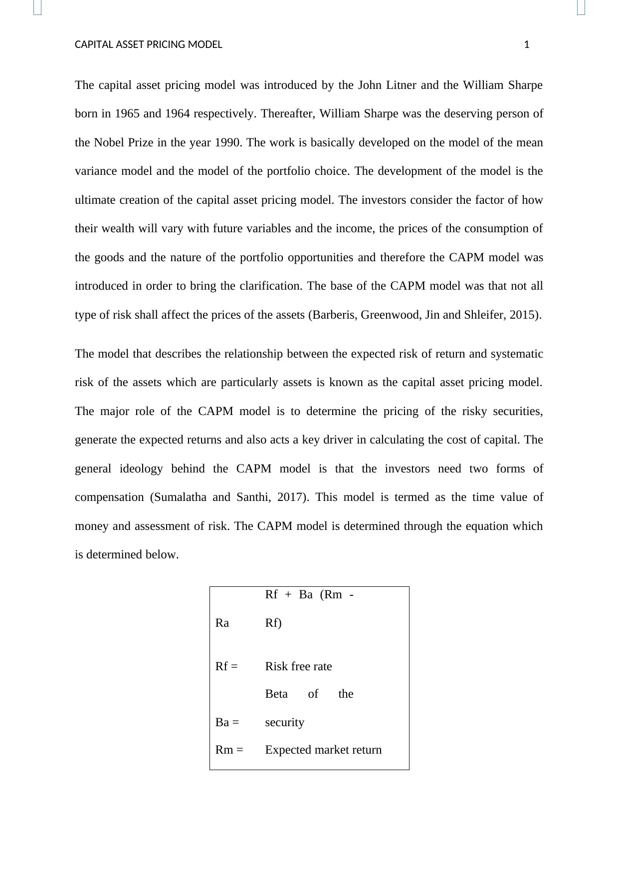
money and assessment of risk. The CAPM model is determined through the equation which
is determined below.
Ra
Rf + Ba (Rm -
Rf)
Rf = Risk free rate
Ba =
Beta of the
security
Rm = Expected market return
The capital asset pricing model was introduced by the John Litner and the William Sharpe
born in 1965 and 1964 respectively. Thereafter, William Sharpe was the deserving person of
the Nobel Prize in the year 1990. The work is basically developed on the model of the mean
variance model and the model of the portfolio choice. The development of the model is the
ultimate creation of the capital asset pricing model. The investors consider the factor of how
their wealth will vary with future variables and the income, the prices of the consumption of
the goods and the nature of the portfolio opportunities and therefore the CAPM model was
introduced in order to bring the clarification. The base of the CAPM model was that not all
type of risk shall affect the prices of the assets (Barberis, Greenwood, Jin and Shleifer, 2015).
The model that describes the relationship between the expected risk of return and systematic
risk of the assets which are particularly assets is known as the capital asset pricing model.
The major role of the CAPM model is to determine the pricing of the risky securities,
generate the expected returns and also acts a key driver in calculating the cost of capital. The
general ideology behind the CAPM model is that the investors need two forms of
compensation (Sumalatha and Santhi, 2017). This model is termed as the time value of
money and assessment of risk. The CAPM model is determined through the equation which
is determined below.
Ra
Rf + Ba (Rm -
Rf)
Rf = Risk free rate
Ba =
Beta of the
security
Rm = Expected market return
CAPITAL ASSET PRICING MODEL 2
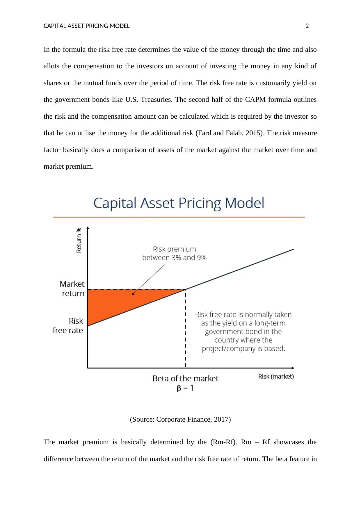
In the formula the risk free rate determines the value of the money through the time and also
allots the compensation to the investors on account of investing the money in any kind of
shares or the mutual funds over the period of time. The risk free rate is customarily yield on
the government bonds like U.S. Treasuries. The second half of the CAPM formula outlines
the risk and the compensation amount can be calculated which is required by the investor so
that he can utilise the money for the additional risk (Fard and Falah, 2015). The risk measure
factor basically does a comparison of assets of the market against the market over time and
market premium.
(Source: Corporate Finance, 2017)
The market premium is basically determined by the (Rm-Rf). Rm – Rf showcases the
difference between the return of the market and the risk free rate of return. The beta feature in
⊘ This is a preview!⊘
Do you want full access?
Subscribe today to unlock all pages.
Trusted by 1+ million students worldwide
CAPITAL ASSET PRICING MODEL 3
this formula reflects the risk factor of an asset with the total risk of the market and the volatile
nature of the asset can also be assessed easily (Bao, Diks and Li, 2018). The main purpose of
the formula is to explicitly determine the correlation between the two above factors.
For example the risk free rate of return is 3%, and the beta value of the stock is 3. The
expected market return over the period is 12%, therefore the market risk premium is (12-3)
which is 9% after getting the difference of the risk free rate of return and the expected market
return.
If all the figures are plugged in than the expected return of the stock is 0.29 or 29%
0.03 + [3*(0.12-0.03)]
There are certain assumptions of the CAPM which are as follows. The CAPM model was
extended by Markowitz which was initially introduced. He put forward his argument that the
investors are risk taker investors. The investment made by the investors is basically the
choice between a portfolio by having a trade-off between the risk and the return for the one
investment period (Fernandez, 2015). The investors choose those portfolios that present the
low variance and provide the specific expected return and therefore the model is known as
Markowitz model.
Paraphrase This Document
Need a fresh take? Get an instant paraphrase of this document with our AI Paraphraser
CAPITAL ASSET PRICING MODEL 4
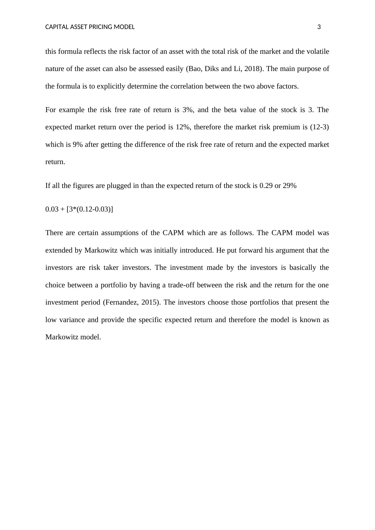
(Source: Accounting Explained, 2017)
Figure 1 says that the CAPM with the amalgamation of the effective frontier and the
extended line for the risk free return point on the y axis. With the help of the standard
deviation the risk of the portfolio can be assessed and the same has been shown on the
horizontal axis.
The inequality of borrowing and the rates determined for the purpose of lending and the same
were outlined by the Friend and Blume 1970 (Campbell, Giglio, Polk and Turley, 2018). The
plausible cause of the difference between the risk and the return feature of New York Stock
Exchange Securities and the assumptions of the Capital asset pricing model is the inequality
between the above two factors. The argument by the authors is about the inequality between
the borrowing from the investor and the lending rates will ultimately result in a risk return
trade off.
The second logic of the assumption of the riskless borrowing and the lending becomes
unrealistic. Black who was born in the year 1972 developed a CAPM model under which he
CAPITAL ASSET PRICING MODEL 5
did not include the above assumption. His idea of setting up the portfolio is that the mean
variance efficient portfolio can be obtained with the help of the short selling of the risky
assets (Fan, Furger and Xiu, 2016).
Again the next assumption of the CAPM model was the divisibility of all the financial assets
fully where the investors have the choice to buy and sell as much more or less securities they
wanted to. Moreover the time period of the selling of the securities was also not fixed and the
same was sold at the market price. Shahzad, S.J.H., Khalid, S. and Ameer, S., (2016)
The major difference between the model of the Sharpe and the linter against the Black was
that in case of the Sharpe-Linter the return was the return is free from the interest but in case
of the Black the return allows the premium and the beta of the market to be positive. Yet the
assumptions made by the Black were also unrealistic in nature. The efficient portfolio does
not exist because there is no risky asset and no unrestricted shorts selling of the risky asset
and therefore there is lack of relationship between the market beta and CAPM. Therefore the
CAPM model is based on the different assumptions (Mazzola and Gerace, 2015).
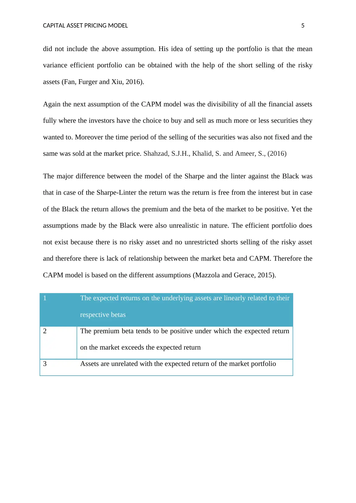
1 The expected returns on the underlying assets are linearly related to their
respective betas
2 The premium beta tends to be positive under which the expected return
on the market exceeds the expected return
3 Assets are unrelated with the expected return of the market portfolio
did not include the above assumption. His idea of setting up the portfolio is that the mean
variance efficient portfolio can be obtained with the help of the short selling of the risky
assets (Fan, Furger and Xiu, 2016).
Again the next assumption of the CAPM model was the divisibility of all the financial assets
fully where the investors have the choice to buy and sell as much more or less securities they
wanted to. Moreover the time period of the selling of the securities was also not fixed and the
same was sold at the market price. Shahzad, S.J.H., Khalid, S. and Ameer, S., (2016)
The major difference between the model of the Sharpe and the linter against the Black was
that in case of the Sharpe-Linter the return was the return is free from the interest but in case
of the Black the return allows the premium and the beta of the market to be positive. Yet the
assumptions made by the Black were also unrealistic in nature. The efficient portfolio does
not exist because there is no risky asset and no unrestricted shorts selling of the risky asset
and therefore there is lack of relationship between the market beta and CAPM. Therefore the
CAPM model is based on the different assumptions (Mazzola and Gerace, 2015).
1 The expected returns on the underlying assets are linearly related to their
respective betas
2 The premium beta tends to be positive under which the expected return
on the market exceeds the expected return
3 Assets are unrelated with the expected return of the market portfolio
⊘ This is a preview!⊘
Do you want full access?
Subscribe today to unlock all pages.
Trusted by 1+ million students worldwide
CAPITAL ASSET PRICING MODEL 6
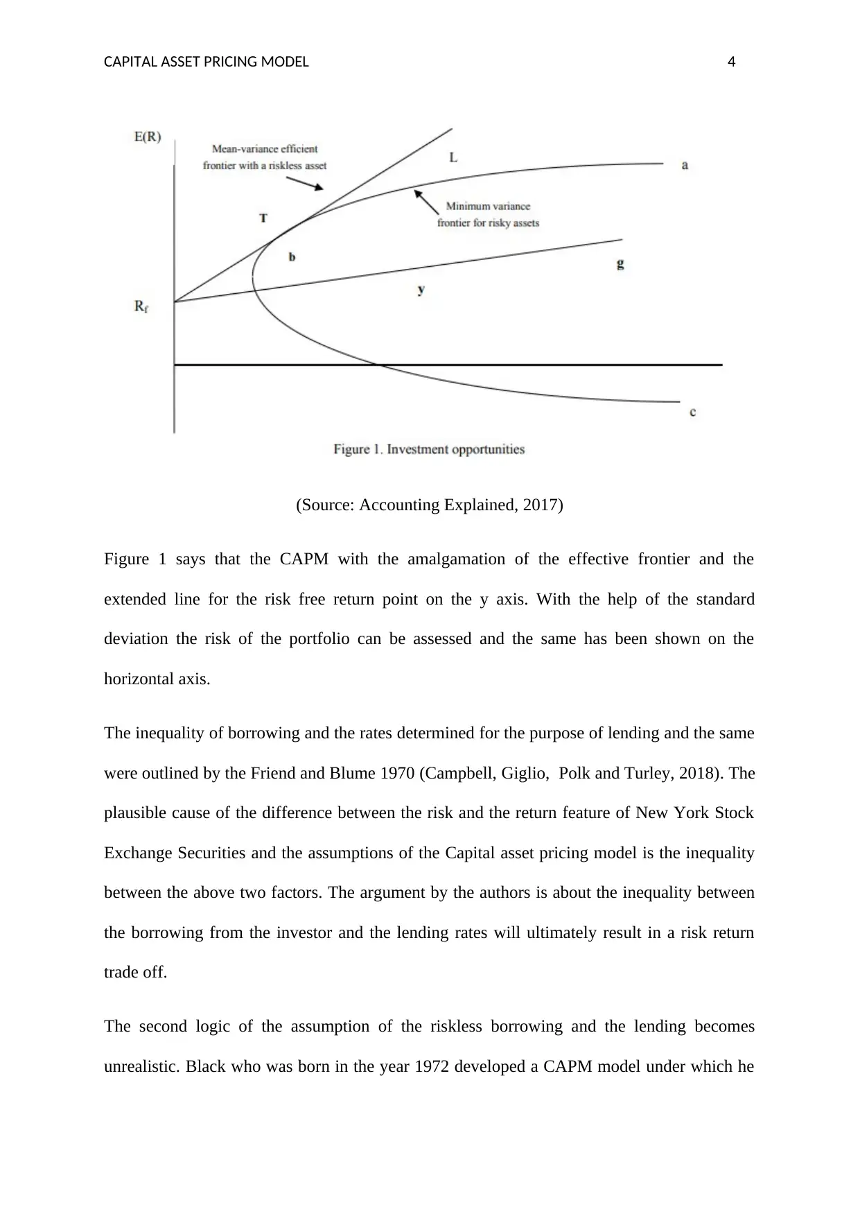
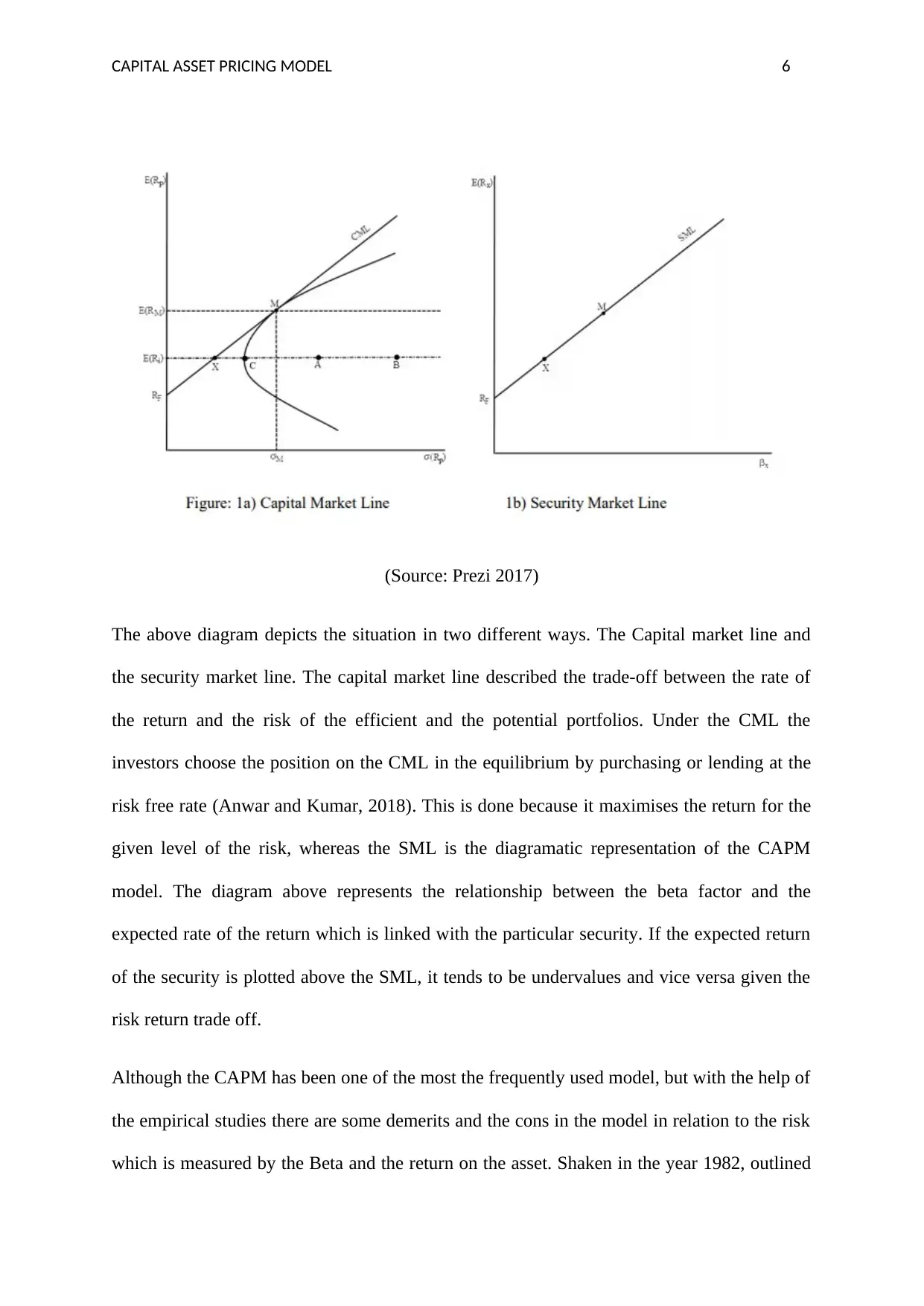
(Source: Prezi 2017)
The above diagram depicts the situation in two different ways. The Capital market line and
the security market line. The capital market line described the trade-off between the rate of
the return and the risk of the efficient and the potential portfolios. Under the CML the
investors choose the position on the CML in the equilibrium by purchasing or lending at the
risk free rate (Anwar and Kumar, 2018). This is done because it maximises the return for the
given level of the risk, whereas the SML is the diagramatic representation of the CAPM
model. The diagram above represents the relationship between the beta factor and the
expected rate of the return which is linked with the particular security. If the expected return
of the security is plotted above the SML, it tends to be undervalues and vice versa given the
risk return trade off.
Although the CAPM has been one of the most the frequently used model, but with the help of
the empirical studies there are some demerits and the cons in the model in relation to the risk
which is measured by the Beta and the return on the asset. Shaken in the year 1982, outlined
Paraphrase This Document
Need a fresh take? Get an instant paraphrase of this document with our AI Paraphraser
CAPITAL ASSET PRICING MODEL 7
his argument on the fact that CAPM model is not truly testable. According to different
investors in the year after 1982, the CAPM model was found as non-testable unless the
market portfolios of all the assets are used in the empirical test (Bendob, Chikhi and
Bennaceur, 2017).
The CAPM has been criticized in many researches and the observations because of the major
assumptions which rely on the two features which are risk free borrowing and lending.
Furthermore, according to the Fama and French there are specific industries for which the
CAPM model did not work at all. The estimates for the cost of equity capital are covered with
errors of more than 3.5% per year. The estimates are not accurate for individual firms and the
projects. There are certain unrealistic assumptions, because of which the CAPM fails due to
the factors for example one period investment, unrestricted risk free borrowing and lending
(Xiao, Faff, Gharghori and Min, 2017)
There are several extensions to the CAPM model from the one it was introduced. The journey
of the CAPM through different versions is states below. Fama and French propose the third
model named as the three factor model. In their model there was an addition of the two
factors such which enhanced the CAPM model in a better manner. The critical factor that
helps to run the three factor model is the size and the market equity. However, at times the
market risk is also considered. Empirically, they provide evidence on the covariance. The
covariance of the small firms is literally high and in case of the large firms the case is reverse.
Further, the stocks are measured by the book to the market ratio (Ready Ratios, 2016).
Merton introduced the ICAPM model in the year 1973. Merton’s inter temporal capital asset
pricing model is an extension of the CAPM. The ICAPM has a different version of the
assumption about the objectives of the investor. Under this CAPM model, investors are
concerned only about the wealth which is obtained by the portfolio at the end of the current
CAPITAL ASSET PRICING MODEL 8
year. But under the ICAPM model the renewed version of the CAPM model the investors and
the stakeholders care about not only the end of the period pay off but also the future
possibilities and the opportunities to consume or invest this pay off. The investors consider
the factor of how their wealth will fluctuate with future variables and the income, the prices
of the consumption of the goods and the nature of the portfolio opportunities (Prezi. 2017).
Lucas who introduced the model in the year 1978 extended the traditional CAPM into the
CCAPM commonly known as the Consumption Capital Asset Pricing Model. This model
describes the direct relationship between the consumption and the stock returns and therefore
it relies upon the aggregate consumption in order to have an analysis and the understanding
of the future asset prices unlike the traditional CAPM Model which links the market’s
portfolio return (Finance Formulas, 2016).
The CAPM model has the numerous advantages over the other methods of calculating the
return and the advantages will surely explain why it has been popular for more than 40 years.
The best feature of the CAPM model is that it considers only the systematic risk and reflects
the reality in which major number of the investors has a wide range of the portfolios from
which the unsystematic risk has been totally eliminated and eradicated.
The CAPM model is the theoretical equation between the required rate of return and the
systematic risk which has been forwarded for the purpose of the future empirical research and
the testing procedures (Accounting Explained, 2017).
In terms of the calculation of the cost of the equity the CAPM model is considered better than
the Dividend Growth Model as it explicitly considers the platform of the systematic risk in
association with the entire stock market.
⊘ This is a preview!⊘
Do you want full access?
Subscribe today to unlock all pages.
Trusted by 1+ million students worldwide
CAPITAL ASSET PRICING MODEL 9
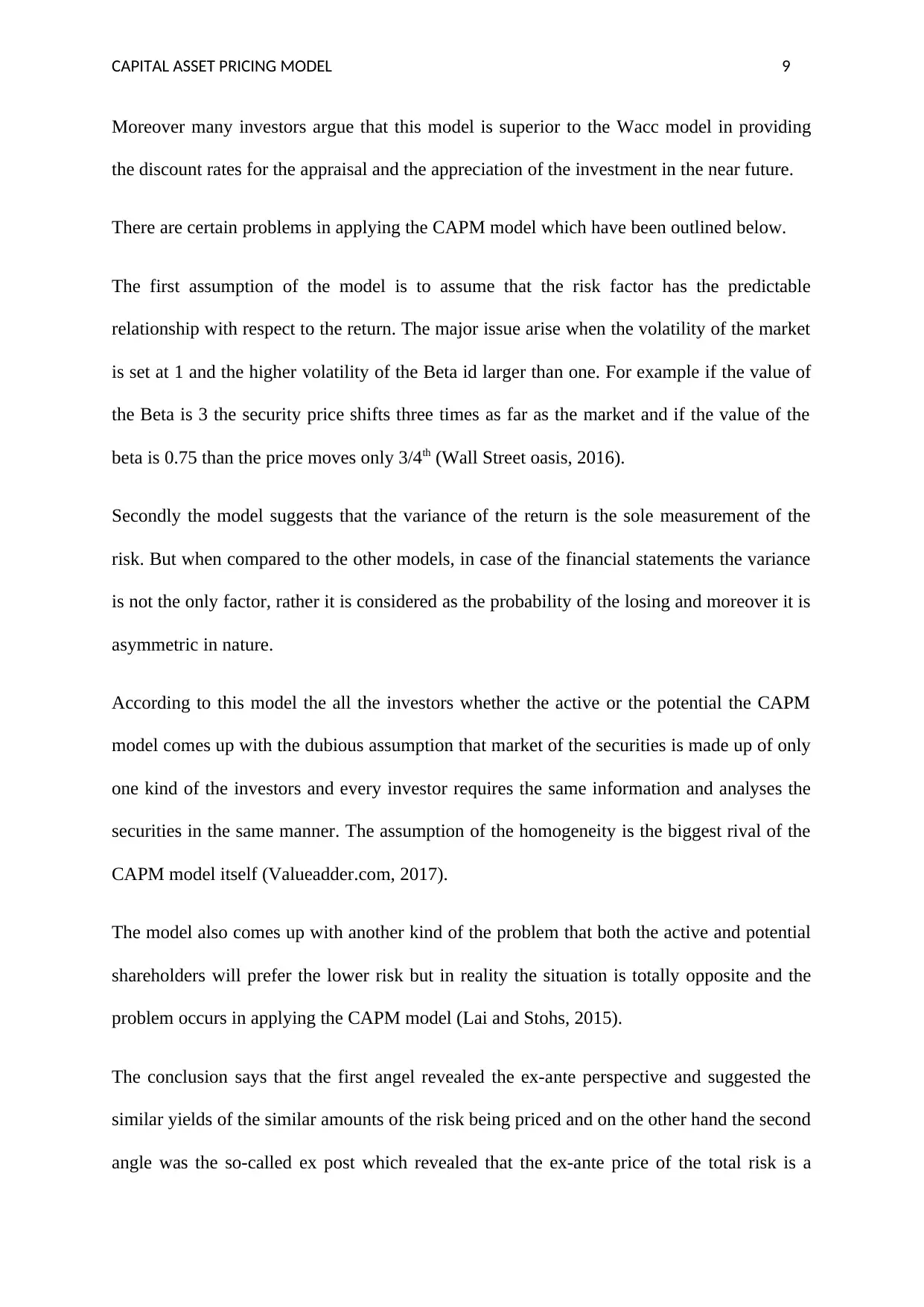
Moreover many investors argue that this model is superior to the Wacc model in providing
the discount rates for the appraisal and the appreciation of the investment in the near future.
There are certain problems in applying the CAPM model which have been outlined below.
The first assumption of the model is to assume that the risk factor has the predictable
relationship with respect to the return. The major issue arise when the volatility of the market
is set at 1 and the higher volatility of the Beta id larger than one. For example if the value of
the Beta is 3 the security price shifts three times as far as the market and if the value of the
beta is 0.75 than the price moves only 3/4th (Wall Street oasis, 2016).
Secondly the model suggests that the variance of the return is the sole measurement of the
risk. But when compared to the other models, in case of the financial statements the variance
is not the only factor, rather it is considered as the probability of the losing and moreover it is
asymmetric in nature.
According to this model the all the investors whether the active or the potential the CAPM
model comes up with the dubious assumption that market of the securities is made up of only
one kind of the investors and every investor requires the same information and analyses the
securities in the same manner. The assumption of the homogeneity is the biggest rival of the
CAPM model itself (Valueadder.com, 2017).
The model also comes up with another kind of the problem that both the active and potential
shareholders will prefer the lower risk but in reality the situation is totally opposite and the
problem occurs in applying the CAPM model (Lai and Stohs, 2015).
The conclusion says that the first angel revealed the ex-ante perspective and suggested the
similar yields of the similar amounts of the risk being priced and on the other hand the second
angle was the so-called ex post which revealed that the ex-ante price of the total risk is a
Paraphrase This Document
Need a fresh take? Get an instant paraphrase of this document with our AI Paraphraser
CAPITAL ASSET PRICING MODEL 10
function of the revised ex post price. These assumptions are not supportive to the paradigm. It
follows directly from the CAOM;s own assumption that if in the situation of the equilibrium
the investors price only the non-diversifiable risks then the fair ex ante price for the total risk
of the asset shall be eventually higher. Therefore from the above essay in my opinion though
the model started to establish itself around 40 years ago there are certain critiques and the
problems in applying the CAPM model correctly to determine the rate of return. Hence, the
investors may consider other models as well to get a variance of the model and the
comparative analysis so that they can invest accordingly.
CAPITAL ASSET PRICING MODEL 11
References
Accounting Explained, (2017) what is Capital Asset Pricing Model (CAPM)? [Online]
Available from https://accountingexplained.com/capital/equity-valuation/capital-asset-
pricing-model [Accessed on 4th September 2018]
Anwar, M. and Kumar, S., (2018) Sectoral Robustness of Asset Pricing Models: Evidence
from the Indian Capital Market. Indian Journal of Commerce and Management Studies, 9(2),
pp.42-50.
Bao, T., Diks, C. and Li, H., (2018) A generalized CAPM model with asymmetric power
distributed errors with an application to portfolio construction. Economic Modelling, 68,
pp.611-621.
Barberis, N., Greenwood, R., Jin, L. and Shleifer, A., (2015) X-CAPM: An extrapolative
capital asset pricing model. Journal of financial economics, 115(1), pp.1-24.
Bendob, A., Chikhi, M. and Bennaceur, F., (2017) Testing the CAPM-GARCH Models in the
GCC-Wide Equity Sectors. Asian Journal of Economic Modelling, 5(4), pp.413-430.
Campbell, J.Y., Giglio, S., Polk, C. and Turley, R., (2018) An intertemporal CAPM with
stochastic volatility. Journal of Financial Economics, 128(2), pp.207-233.
Fan, J., Furger, A. and Xiu, D., (2016) Incorporating global industrial classification standard
into portfolio allocation: A simple factor-based large covariance matrix estimator with high-
frequency data. Journal of Business & Economic Statistics, 34(4), pp.489-503.
Fard, H.V. and Falah, A.B., (2015) A New Modified CAPM Model: The Two Beta
CAPM. Jurnal UMP Social Sciences and Technology Management Vol, 3(1).
⊘ This is a preview!⊘
Do you want full access?
Subscribe today to unlock all pages.
Trusted by 1+ million students worldwide
1 out of 14
Related Documents


Your All-in-One AI-Powered Toolkit for Academic Success.
+13062052269
info@desklib.com
Available 24*7 on WhatsApp / Email
![[object Object]](/_next/static/media/star-bottom.7253800d.svg)
Unlock your academic potential
Copyright © 2020–2026 A2Z Services. All Rights Reserved. Developed and managed by ZUCOL.