Capital Budgeting and Project Evaluation: Risk Analysis and Cash Flow
VerifiedAdded on 2021/06/22
|13
|3612
|26
Report
AI Summary
This report delves into the core concepts of capital budgeting and project evaluation, essential for sound financial decision-making within organizations. It begins with an introduction to capital budgeting, outlining its significance in assessing project investments and estimating key financial metrics. The report then explores incremental and operating cash flows, along with depreciation methods and working capital considerations. A significant portion of the report is dedicated to risk analysis and project evaluation, including scenario analysis with cash flow projections, and sensitivity analyses under base, best, and worst-case scenarios. The report also incorporates a comparative analysis to highlight the impact of different scenarios on project outcomes. Overall, the report provides a practical application of financial tools to assess project feasibility and profitability, with specific examples related to a production unit.
[Due Date]
Business Finance
Capital Budgeting and
Project Evaluation
[Student Name]
Business Finance
Capital Budgeting and
Project Evaluation
[Student Name]
Paraphrase This Document
Need a fresh take? Get an instant paraphrase of this document with our AI Paraphraser
Index Title Page No
1 Introduction 1
2 Part 1 - Capital budgeting 1
3 Part 2: Risk Analysis and Project Evaluation 3
3.1 Scenario Analysis with Cash Flow 3
3.2 Sensitivity of the project 6
3.2.1 Case 1: Base Case 6
3.2.2 Case 2: Best Case 7
3.2.3 Case 3: Worst Case 8
4 Comparative Analysis 9
5 Conclusion 10
Reference 11
1
CAPITAL BUDGETING AND PROJECT EVALUATION
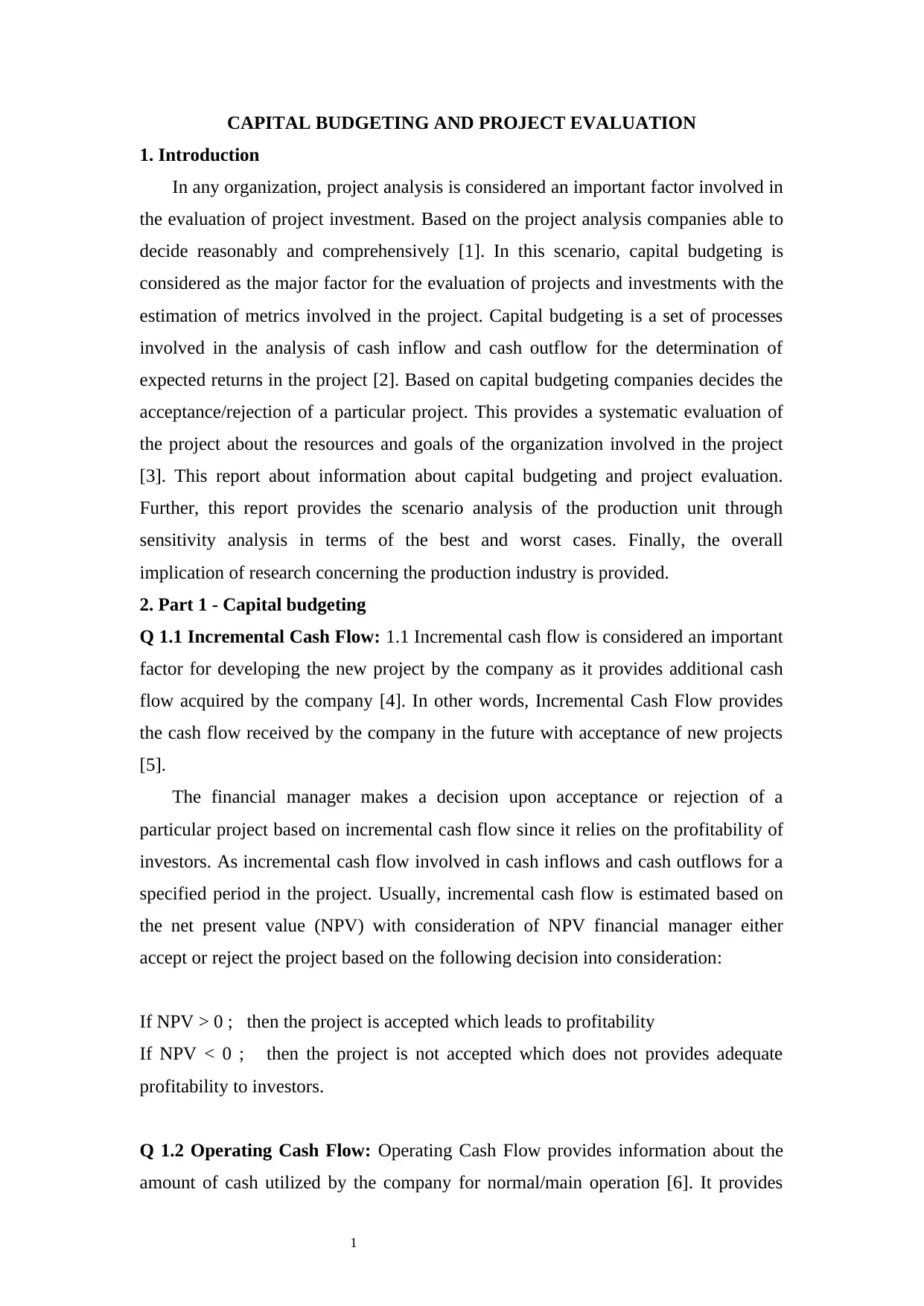
1. Introduction
In any organization, project analysis is considered an important factor involved in
the evaluation of project investment. Based on the project analysis companies able to
decide reasonably and comprehensively [1]. In this scenario, capital budgeting is
considered as the major factor for the evaluation of projects and investments with the
estimation of metrics involved in the project. Capital budgeting is a set of processes
involved in the analysis of cash inflow and cash outflow for the determination of
expected returns in the project [2]. Based on capital budgeting companies decides the
acceptance/rejection of a particular project. This provides a systematic evaluation of
the project about the resources and goals of the organization involved in the project
[3]. This report about information about capital budgeting and project evaluation.
Further, this report provides the scenario analysis of the production unit through
sensitivity analysis in terms of the best and worst cases. Finally, the overall
implication of research concerning the production industry is provided.
2. Part 1 - Capital budgeting
Q 1.1 Incremental Cash Flow: 1.1 Incremental cash flow is considered an important
factor for developing the new project by the company as it provides additional cash
flow acquired by the company [4]. In other words, Incremental Cash Flow provides
the cash flow received by the company in the future with acceptance of new projects
[5].
The financial manager makes a decision upon acceptance or rejection of a
particular project based on incremental cash flow since it relies on the profitability of
investors. As incremental cash flow involved in cash inflows and cash outflows for a
specified period in the project. Usually, incremental cash flow is estimated based on
the net present value (NPV) with consideration of NPV financial manager either
accept or reject the project based on the following decision into consideration:
If NPV > 0 ; then the project is accepted which leads to profitability
If NPV < 0 ; then the project is not accepted which does not provides adequate
profitability to investors.
Q 1.2 Operating Cash Flow: Operating Cash Flow provides information about the
amount of cash utilized by the company for normal/main operation [6]. It provides
CAPITAL BUDGETING AND PROJECT EVALUATION
1. Introduction
In any organization, project analysis is considered an important factor involved in
the evaluation of project investment. Based on the project analysis companies able to
decide reasonably and comprehensively [1]. In this scenario, capital budgeting is
considered as the major factor for the evaluation of projects and investments with the
estimation of metrics involved in the project. Capital budgeting is a set of processes
involved in the analysis of cash inflow and cash outflow for the determination of
expected returns in the project [2]. Based on capital budgeting companies decides the
acceptance/rejection of a particular project. This provides a systematic evaluation of
the project about the resources and goals of the organization involved in the project
[3]. This report about information about capital budgeting and project evaluation.
Further, this report provides the scenario analysis of the production unit through
sensitivity analysis in terms of the best and worst cases. Finally, the overall
implication of research concerning the production industry is provided.
2. Part 1 - Capital budgeting
Q 1.1 Incremental Cash Flow: 1.1 Incremental cash flow is considered an important
factor for developing the new project by the company as it provides additional cash
flow acquired by the company [4]. In other words, Incremental Cash Flow provides
the cash flow received by the company in the future with acceptance of new projects
[5].
The financial manager makes a decision upon acceptance or rejection of a
particular project based on incremental cash flow since it relies on the profitability of
investors. As incremental cash flow involved in cash inflows and cash outflows for a
specified period in the project. Usually, incremental cash flow is estimated based on
the net present value (NPV) with consideration of NPV financial manager either
accept or reject the project based on the following decision into consideration:
If NPV > 0 ; then the project is accepted which leads to profitability
If NPV < 0 ; then the project is not accepted which does not provides adequate
profitability to investors.
Q 1.2 Operating Cash Flow: Operating Cash Flow provides information about the
amount of cash utilized by the company for normal/main operation [6]. It provides
⊘ This is a preview!⊘
Do you want full access?
Subscribe today to unlock all pages.
Trusted by 1+ million students worldwide
2
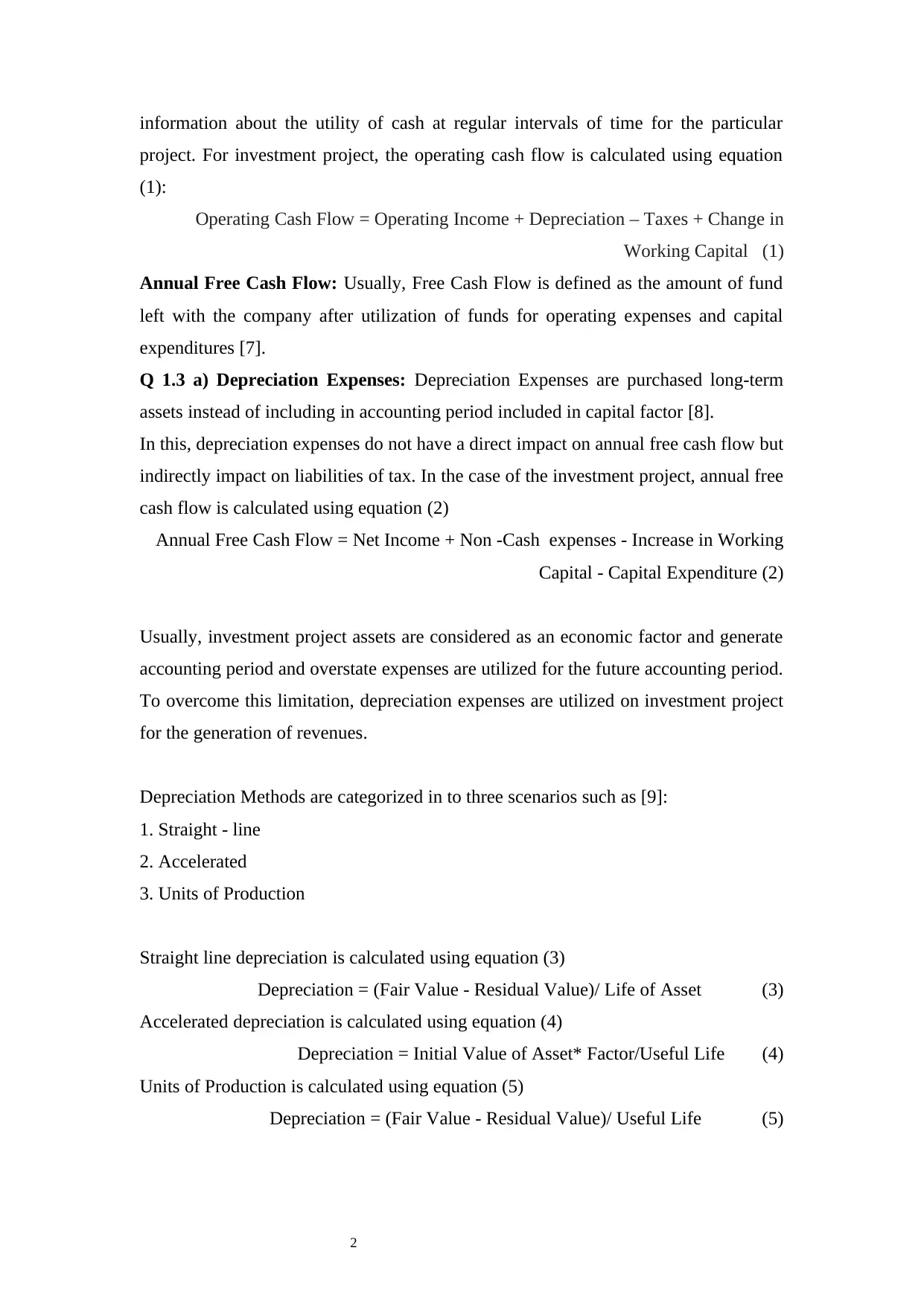
information about the utility of cash at regular intervals of time for the particular
project. For investment project, the operating cash flow is calculated using equation
(1):
Operating Cash Flow = Operating Income + Depreciation – Taxes + Change in
Working Capital (1)
Annual Free Cash Flow: Usually, Free Cash Flow is defined as the amount of fund
left with the company after utilization of funds for operating expenses and capital
expenditures [7].
Q 1.3 a) Depreciation Expenses: Depreciation Expenses are purchased long-term
assets instead of including in accounting period included in capital factor [8].
In this, depreciation expenses do not have a direct impact on annual free cash flow but
indirectly impact on liabilities of tax. In the case of the investment project, annual free
cash flow is calculated using equation (2)
Annual Free Cash Flow = Net Income + Non -Cash expenses - Increase in Working
Capital - Capital Expenditure (2)
Usually, investment project assets are considered as an economic factor and generate
accounting period and overstate expenses are utilized for the future accounting period.
To overcome this limitation, depreciation expenses are utilized on investment project
for the generation of revenues.
Depreciation Methods are categorized in to three scenarios such as [9]:
1. Straight - line
2. Accelerated
3. Units of Production
Straight line depreciation is calculated using equation (3)
Depreciation = (Fair Value - Residual Value)/ Life of Asset (3)
Accelerated depreciation is calculated using equation (4)
Depreciation = Initial Value of Asset* Factor/Useful Life (4)
Units of Production is calculated using equation (5)
Depreciation = (Fair Value - Residual Value)/ Useful Life (5)
Paraphrase This Document
Need a fresh take? Get an instant paraphrase of this document with our AI Paraphraser
3
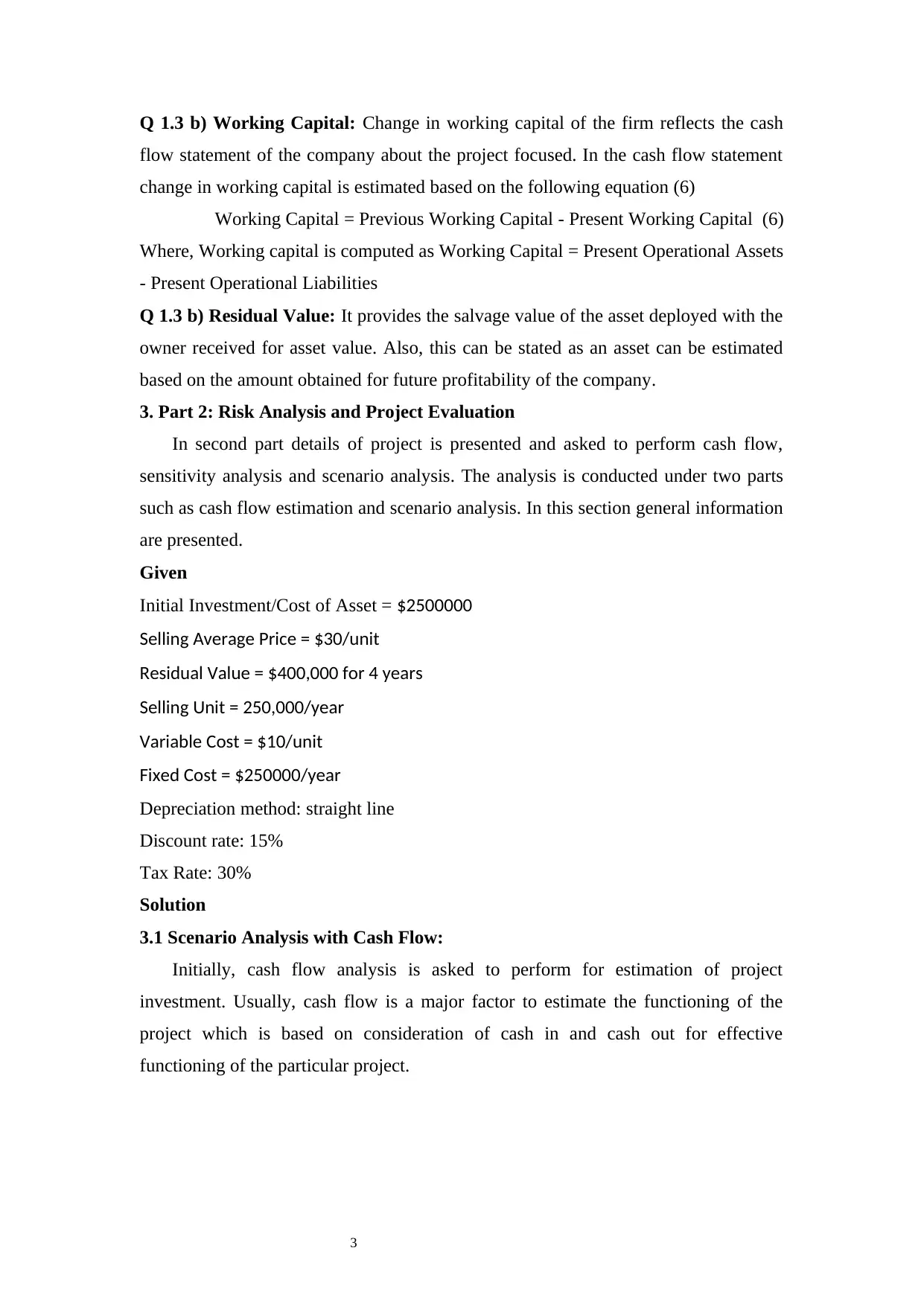
Q 1.3 b) Working Capital: Change in working capital of the firm reflects the cash
flow statement of the company about the project focused. In the cash flow statement
change in working capital is estimated based on the following equation (6)
Working Capital = Previous Working Capital - Present Working Capital (6)
Where, Working capital is computed as Working Capital = Present Operational Assets
- Present Operational Liabilities
Q 1.3 b) Residual Value: It provides the salvage value of the asset deployed with the
owner received for asset value. Also, this can be stated as an asset can be estimated
based on the amount obtained for future profitability of the company.
3. Part 2: Risk Analysis and Project Evaluation
In second part details of project is presented and asked to perform cash flow,
sensitivity analysis and scenario analysis. The analysis is conducted under two parts
such as cash flow estimation and scenario analysis. In this section general information
are presented.
Given
Initial Investment/Cost of Asset = $2500000
Selling Average Price = $30/unit
Residual Value = $400,000 for 4 years
Selling Unit = 250,000/year
Variable Cost = $10/unit
Fixed Cost = $250000/year
Depreciation method: straight line
Discount rate: 15%
Tax Rate: 30%
Solution
3.1 Scenario Analysis with Cash Flow:
Initially, cash flow analysis is asked to perform for estimation of project
investment. Usually, cash flow is a major factor to estimate the functioning of the
project which is based on consideration of cash in and cash out for effective
functioning of the particular project.
4
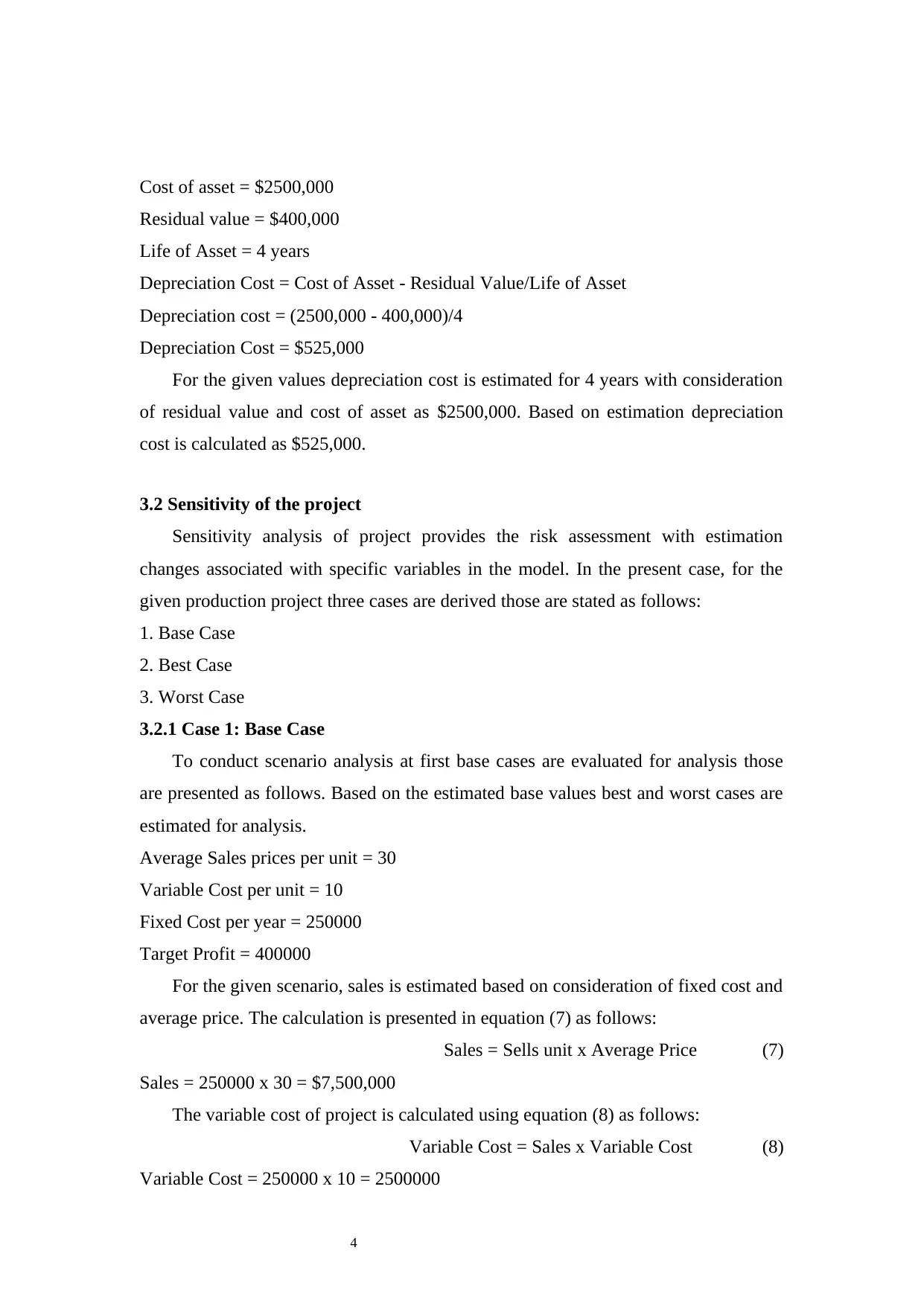
Cost of asset = $2500,000
Residual value = $400,000
Life of Asset = 4 years
Depreciation Cost = Cost of Asset - Residual Value/Life of Asset
Depreciation cost = (2500,000 - 400,000)/4
Depreciation Cost = $525,000
For the given values depreciation cost is estimated for 4 years with consideration
of residual value and cost of asset as $2500,000. Based on estimation depreciation
cost is calculated as $525,000.
3.2 Sensitivity of the project
Sensitivity analysis of project provides the risk assessment with estimation
changes associated with specific variables in the model. In the present case, for the
given production project three cases are derived those are stated as follows:
1. Base Case
2. Best Case
3. Worst Case
3.2.1 Case 1: Base Case
To conduct scenario analysis at first base cases are evaluated for analysis those
are presented as follows. Based on the estimated base values best and worst cases are
estimated for analysis.
Average Sales prices per unit = 30
Variable Cost per unit = 10
Fixed Cost per year = 250000
Target Profit = 400000
For the given scenario, sales is estimated based on consideration of fixed cost and
average price. The calculation is presented in equation (7) as follows:
Sales = Sells unit x Average Price (7)
Sales = 250000 x 30 = $7,500,000
The variable cost of project is calculated using equation (8) as follows:
Variable Cost = Sales x Variable Cost (8)
Variable Cost = 250000 x 10 = 2500000
⊘ This is a preview!⊘
Do you want full access?
Subscribe today to unlock all pages.
Trusted by 1+ million students worldwide
5
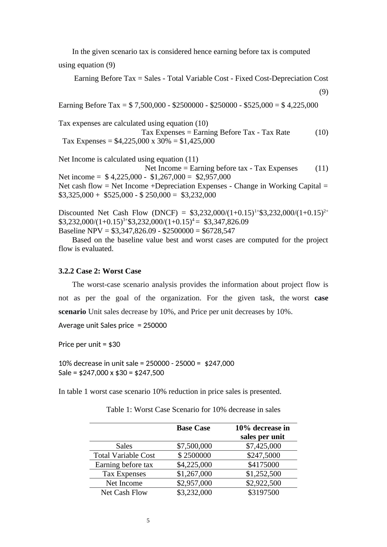
In the given scenario tax is considered hence earning before tax is computed
using equation (9)
Earning Before Tax = Sales - Total Variable Cost - Fixed Cost-Depreciation Cost
(9)
Earning Before Tax = $ 7,500,000 - $2500000 - $250000 - $525,000 = $ 4,225,000
Tax expenses are calculated using equation (10)
Tax Expenses = Earning Before Tax - Tax Rate (10)
Tax Expenses = $4,225,000 x 30% = $1,425,000
Net Income is calculated using equation (11)
Net Income = Earning before tax - Tax Expenses (11)
Net income = $ 4,225,000 - $1,267,000 = $2,957,000
Net cash flow = Net Income +Depreciation Expenses - Change in Working Capital =
$3,325,000 + $525,000 - $ 250,000 = $3,232,000
Discounted Net Cash Flow (DNCF) = $3,232,000/(1+0.15)1+$3,232,000/(1+0.15)2+
$3,232,000/(1+0.15)3+$3,232,000/(1+0.15)4 = $3,347,826.09
Baseline NPV = $3,347,826.09 - $2500000 = $6728,547
Based on the baseline value best and worst cases are computed for the project
flow is evaluated.
3.2.2 Case 2: Worst Case
The worst-case scenario analysis provides the information about project flow is
not as per the goal of the organization. For the given task, the worst case
scenario Unit sales decrease by 10%, and Price per unit decreases by 10%.
Average unit Sales price = 250000
Price per unit = $30
10% decrease in unit sale = 250000 - 25000 = $247,000
Sale = $247,000 x $30 = $247,500
In table 1 worst case scenario 10% reduction in price sales is presented.
Table 1: Worst Case Scenario for 10% decrease in sales
Base Case 10% decrease in
sales per unit
Sales $7,500,000 $7,425,000
Total Variable Cost $ 2500000 $247,5000
Earning before tax $4,225,000 $4175000
Tax Expenses $1,267,000 $1,252,500
Net Income $2,957,000 $2,922,500
Net Cash Flow $3,232,000 $3197500
Paraphrase This Document
Need a fresh take? Get an instant paraphrase of this document with our AI Paraphraser
6
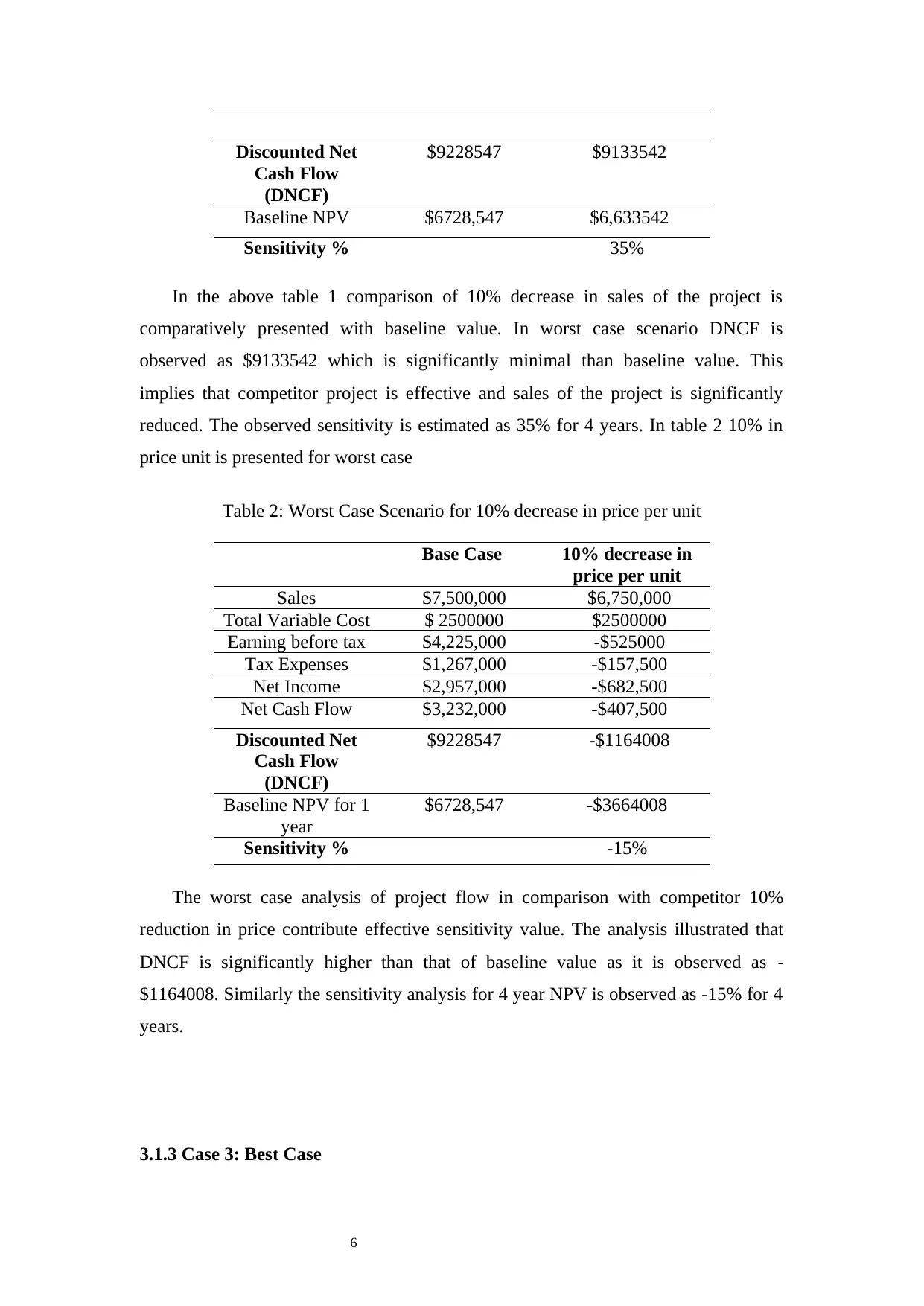
Discounted Net
Cash Flow
(DNCF)
$9228547 $9133542
Baseline NPV $6728,547 $6,633542
Sensitivity % 35%
In the above table 1 comparison of 10% decrease in sales of the project is
comparatively presented with baseline value. In worst case scenario DNCF is
observed as $9133542 which is significantly minimal than baseline value. This
implies that competitor project is effective and sales of the project is significantly
reduced. The observed sensitivity is estimated as 35% for 4 years. In table 2 10% in
price unit is presented for worst case
Table 2: Worst Case Scenario for 10% decrease in price per unit
Base Case 10% decrease in
price per unit
Sales $7,500,000 $6,750,000
Total Variable Cost $ 2500000 $2500000
Earning before tax $4,225,000 -$525000
Tax Expenses $1,267,000 -$157,500
Net Income $2,957,000 -$682,500
Net Cash Flow $3,232,000 -$407,500
Discounted Net
Cash Flow
(DNCF)
$9228547 -$1164008
Baseline NPV for 1
year
$6728,547 -$3664008
Sensitivity % -15%
The worst case analysis of project flow in comparison with competitor 10%
reduction in price contribute effective sensitivity value. The analysis illustrated that
DNCF is significantly higher than that of baseline value as it is observed as -
$1164008. Similarly the sensitivity analysis for 4 year NPV is observed as -15% for 4
years.
3.1.3 Case 3: Best Case
Discounted Net
Cash Flow
(DNCF)
$9228547 $9133542
Baseline NPV $6728,547 $6,633542
Sensitivity % 35%
In the above table 1 comparison of 10% decrease in sales of the project is
comparatively presented with baseline value. In worst case scenario DNCF is
observed as $9133542 which is significantly minimal than baseline value. This
implies that competitor project is effective and sales of the project is significantly
reduced. The observed sensitivity is estimated as 35% for 4 years. In table 2 10% in
price unit is presented for worst case
Table 2: Worst Case Scenario for 10% decrease in price per unit
Base Case 10% decrease in
price per unit
Sales $7,500,000 $6,750,000
Total Variable Cost $ 2500000 $2500000
Earning before tax $4,225,000 -$525000
Tax Expenses $1,267,000 -$157,500
Net Income $2,957,000 -$682,500
Net Cash Flow $3,232,000 -$407,500
Discounted Net
Cash Flow
(DNCF)
$9228547 -$1164008
Baseline NPV for 1
year
$6728,547 -$3664008
Sensitivity % -15%
The worst case analysis of project flow in comparison with competitor 10%
reduction in price contribute effective sensitivity value. The analysis illustrated that
DNCF is significantly higher than that of baseline value as it is observed as -
$1164008. Similarly the sensitivity analysis for 4 year NPV is observed as -15% for 4
years.
3.1.3 Case 3: Best Case
7
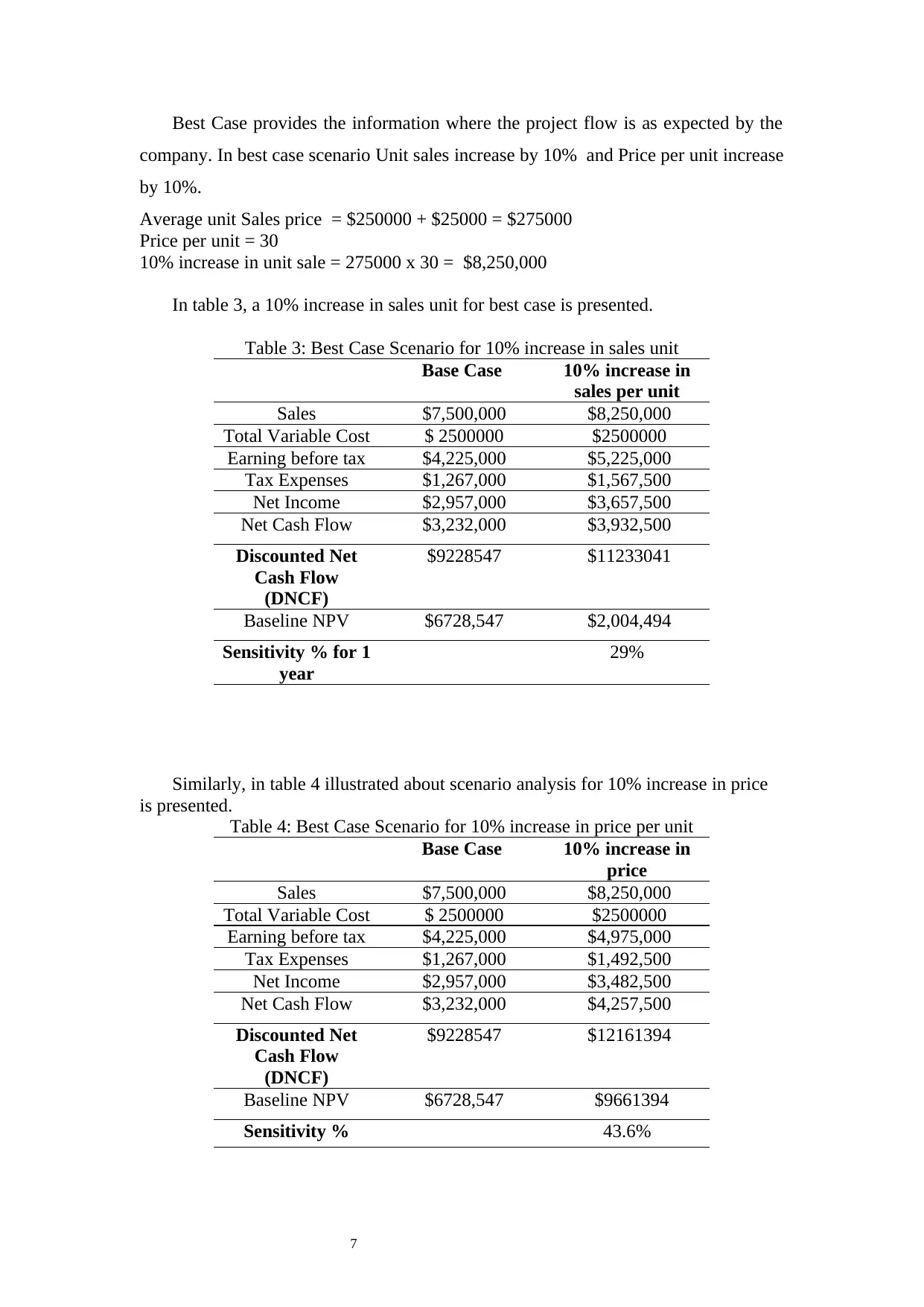
Best Case provides the information where the project flow is as expected by the
company. In best case scenario Unit sales increase by 10% and Price per unit increase
by 10%.
Average unit Sales price = $250000 + $25000 = $275000
Price per unit = 30
10% increase in unit sale = 275000 x 30 = $8,250,000
In table 3, a 10% increase in sales unit for best case is presented.
Table 3: Best Case Scenario for 10% increase in sales unit
Base Case 10% increase in
sales per unit
Sales $7,500,000 $8,250,000
Total Variable Cost $ 2500000 $2500000
Earning before tax $4,225,000 $5,225,000
Tax Expenses $1,267,000 $1,567,500
Net Income $2,957,000 $3,657,500
Net Cash Flow $3,232,000 $3,932,500
Discounted Net
Cash Flow
(DNCF)
$9228547 $11233041
Baseline NPV $6728,547 $2,004,494
Sensitivity % for 1
year
29%
Similarly, in table 4 illustrated about scenario analysis for 10% increase in price
is presented.
Table 4: Best Case Scenario for 10% increase in price per unit
Base Case 10% increase in
price
Sales $7,500,000 $8,250,000
Total Variable Cost $ 2500000 $2500000
Earning before tax $4,225,000 $4,975,000
Tax Expenses $1,267,000 $1,492,500
Net Income $2,957,000 $3,482,500
Net Cash Flow $3,232,000 $4,257,500
Discounted Net
Cash Flow
(DNCF)
$9228547 $12161394
Baseline NPV $6728,547 $9661394
Sensitivity % 43.6%
⊘ This is a preview!⊘
Do you want full access?
Subscribe today to unlock all pages.
Trusted by 1+ million students worldwide
8
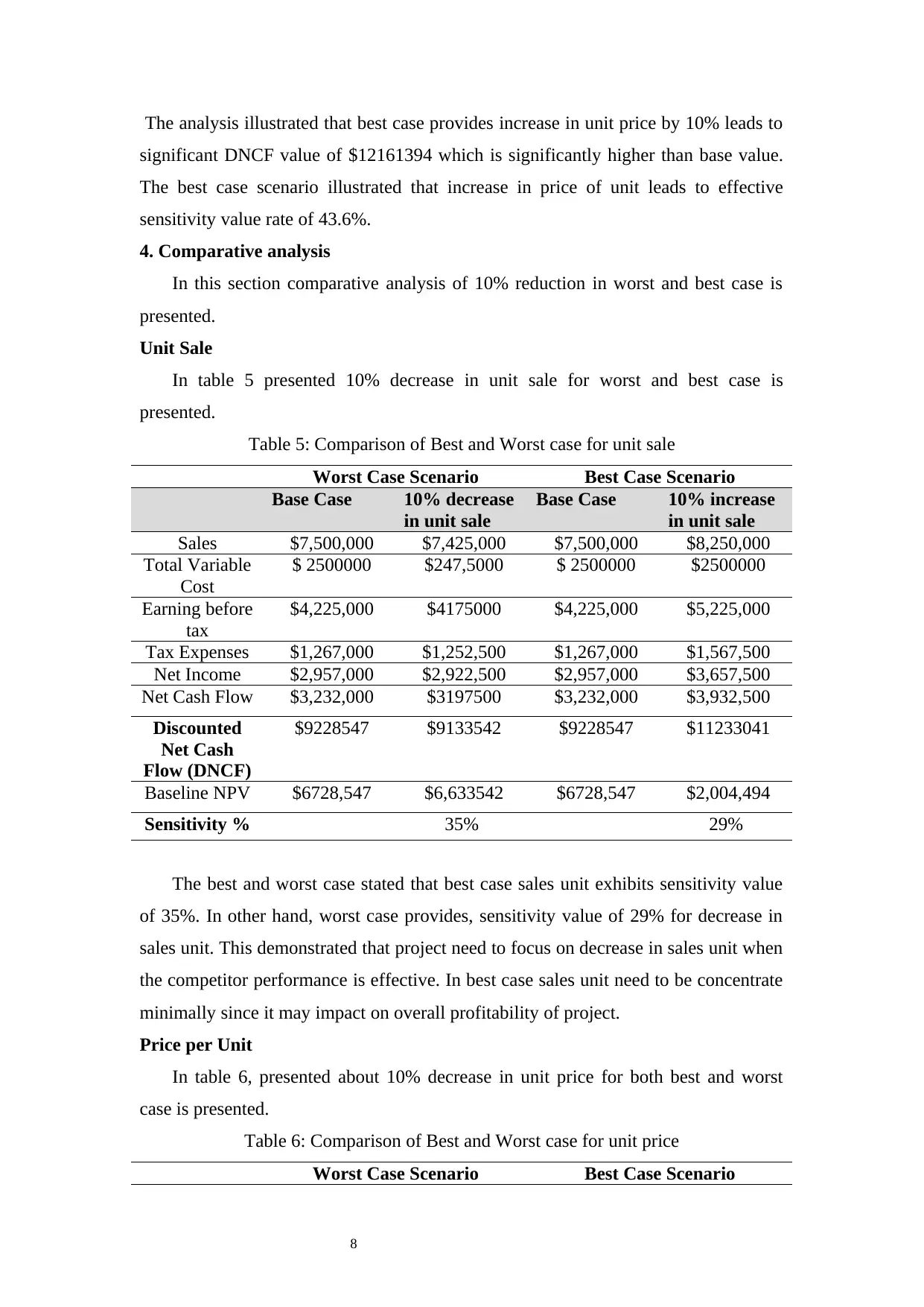
The analysis illustrated that best case provides increase in unit price by 10% leads to
significant DNCF value of $12161394 which is significantly higher than base value.
The best case scenario illustrated that increase in price of unit leads to effective
sensitivity value rate of 43.6%.
4. Comparative analysis
In this section comparative analysis of 10% reduction in worst and best case is
presented.
Unit Sale
In table 5 presented 10% decrease in unit sale for worst and best case is
presented.
Table 5: Comparison of Best and Worst case for unit sale
Worst Case Scenario Best Case Scenario
Base Case 10% decrease
in unit sale
Base Case 10% increase
in unit sale
Sales $7,500,000 $7,425,000 $7,500,000 $8,250,000
Total Variable
Cost
$ 2500000 $247,5000 $ 2500000 $2500000
Earning before
tax
$4,225,000 $4175000 $4,225,000 $5,225,000
Tax Expenses $1,267,000 $1,252,500 $1,267,000 $1,567,500
Net Income $2,957,000 $2,922,500 $2,957,000 $3,657,500
Net Cash Flow $3,232,000 $3197500 $3,232,000 $3,932,500
Discounted
Net Cash
Flow (DNCF)
$9228547 $9133542 $9228547 $11233041
Baseline NPV $6728,547 $6,633542 $6728,547 $2,004,494
Sensitivity % 35% 29%
The best and worst case stated that best case sales unit exhibits sensitivity value
of 35%. In other hand, worst case provides, sensitivity value of 29% for decrease in
sales unit. This demonstrated that project need to focus on decrease in sales unit when
the competitor performance is effective. In best case sales unit need to be concentrate
minimally since it may impact on overall profitability of project.
Price per Unit
In table 6, presented about 10% decrease in unit price for both best and worst
case is presented.
Table 6: Comparison of Best and Worst case for unit price
Worst Case Scenario Best Case Scenario
Paraphrase This Document
Need a fresh take? Get an instant paraphrase of this document with our AI Paraphraser
9
Base Case 10% decrease
in unit price
Base Case 10% increase
in unit price
Sales $7,500,000 $6,750,000 $7,500,000 $8,250,000
Total Variable
Cost
$ 2500000 $2500000 $ 2500000 $2500000
Earning before
tax
$4,225,000 -$525000 $4,225,000 $4,975,000
Tax Expenses $1,267,000 -$157,500 $1,267,000 $1,492,500
Net Income $2,957,000 -$682,500 $2,957,000 $3,482,500
Net Cash Flow $3,232,000 -$407,500 $3,232,000 $4,257,500
Discounted
Net Cash
Flow (DNCF)
$9228547 -$1164008 $9228547 $12161394
Baseline NPV $6728,547 -$3664008 $6728,547 $9661394
Sensitivity % -15% 43.6%
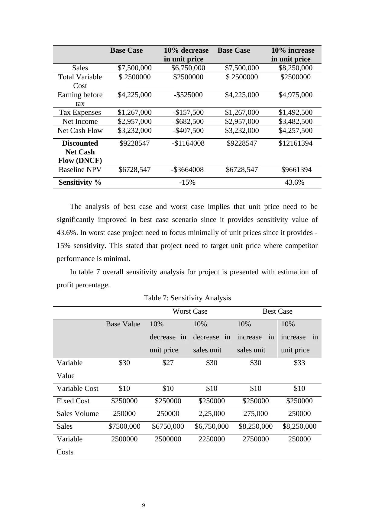
The analysis of best case and worst case implies that unit price need to be
significantly improved in best case scenario since it provides sensitivity value of
43.6%. In worst case project need to focus minimally of unit prices since it provides -
15% sensitivity. This stated that project need to target unit price where competitor
performance is minimal.
In table 7 overall sensitivity analysis for project is presented with estimation of
profit percentage.
Table 7: Sensitivity Analysis
Worst Case Best Case
Base Value 10%
decrease in
unit price
10%
decrease in
sales unit
10%
increase in
sales unit
10%
increase in
unit price
Variable
Value
$30 $27 $30 $30 $33
Variable Cost $10 $10 $10 $10 $10
Fixed Cost $250000 $250000 $250000 $250000 $250000
Sales Volume 250000 250000 2,25,000 275,000 250000
Sales $7500,000 $6750,000 $6,750,000 $8,250,000 $8,250,000
Variable
Costs
2500000 2500000 2250000 2750000 250000
Base Case 10% decrease
in unit price
Base Case 10% increase
in unit price
Sales $7,500,000 $6,750,000 $7,500,000 $8,250,000
Total Variable
Cost
$ 2500000 $2500000 $ 2500000 $2500000
Earning before
tax
$4,225,000 -$525000 $4,225,000 $4,975,000
Tax Expenses $1,267,000 -$157,500 $1,267,000 $1,492,500
Net Income $2,957,000 -$682,500 $2,957,000 $3,482,500
Net Cash Flow $3,232,000 -$407,500 $3,232,000 $4,257,500
Discounted
Net Cash
Flow (DNCF)
$9228547 -$1164008 $9228547 $12161394
Baseline NPV $6728,547 -$3664008 $6728,547 $9661394
Sensitivity % -15% 43.6%
The analysis of best case and worst case implies that unit price need to be
significantly improved in best case scenario since it provides sensitivity value of
43.6%. In worst case project need to focus minimally of unit prices since it provides -
15% sensitivity. This stated that project need to target unit price where competitor
performance is minimal.
In table 7 overall sensitivity analysis for project is presented with estimation of
profit percentage.
Table 7: Sensitivity Analysis
Worst Case Best Case
Base Value 10%
decrease in
unit price
10%
decrease in
sales unit
10%
increase in
sales unit
10%
increase in
unit price
Variable
Value
$30 $27 $30 $30 $33
Variable Cost $10 $10 $10 $10 $10
Fixed Cost $250000 $250000 $250000 $250000 $250000
Sales Volume 250000 250000 2,25,000 275,000 250000
Sales $7500,000 $6750,000 $6,750,000 $8,250,000 $8,250,000
Variable
Costs
2500000 2500000 2250000 2750000 250000
10
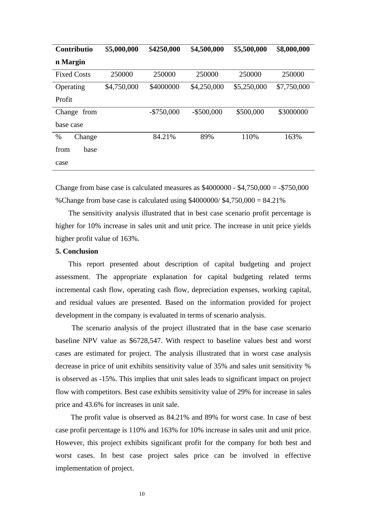
Contributio
n Margin
$5,000,000 $4250,000 $4,500,000 $5,500,000 $8,000,000
Fixed Costs 250000 250000 250000 250000 250000
Operating
Profit
$4,750,000 $4000000 $4,250,000 $5,250,000 $7,750,000
Change from
base case
-$750,000 -$500,000 $500,000 $3000000
% Change
from base
case
84.21% 89% 110% 163%
Change from base case is calculated measures as $4000000 - $4,750,000 = -$750,000
%Change from base case is calculated using $4000000/ $4,750,000 = 84.21%
The sensitivity analysis illustrated that in best case scenario profit percentage is
higher for 10% increase in sales unit and unit price. The increase in unit price yields
higher profit value of 163%.
5. Conclusion
This report presented about description of capital budgeting and project
assessment. The appropriate explanation for capital budgeting related terms
incremental cash flow, operating cash flow, depreciation expenses, working capital,
and residual values are presented. Based on the information provided for project
development in the company is evaluated in terms of scenario analysis.
The scenario analysis of the project illustrated that in the base case scenario
baseline NPV value as $6728,547. With respect to baseline values best and worst
cases are estimated for project. The analysis illustrated that in worst case analysis
decrease in price of unit exhibits sensitivity value of 35% and sales unit sensitivity %
is observed as -15%. This implies that unit sales leads to significant impact on project
flow with competitors. Best case exhibits sensitivity value of 29% for increase in sales
price and 43.6% for increases in unit sale.
The profit value is observed as 84.21% and 89% for worst case. In case of best
case profit percentage is 110% and 163% for 10% increase in sales unit and unit price.
However, this project exhibits significant profit for the company for both best and
worst cases. In best case project sales price can be involved in effective
implementation of project.
⊘ This is a preview!⊘
Do you want full access?
Subscribe today to unlock all pages.
Trusted by 1+ million students worldwide
1 out of 13
Related Documents


Your All-in-One AI-Powered Toolkit for Academic Success.
+13062052269
info@desklib.com
Available 24*7 on WhatsApp / Email
![[object Object]](/_next/static/media/star-bottom.7253800d.svg)
Unlock your academic potential
Copyright © 2020–2026 A2Z Services. All Rights Reserved. Developed and managed by ZUCOL.