Financial Analysis: Capital Budgeting and Cost of Capital for GOGreen

This report presents a detailed financial analysis focused on capital budgeting and the cost of capital. The first part of the report involves a capital budgeting analysis, where the after-tax cash flows, payback period, Net Present Value (NPV), and Profitability Index (PI) are calculated to evaluate the financial viability of an equipment upgrade proposal for GOGreen Motors. The analysis includes sensitivity analysis considering a change in variable costs. The second part of the report delves into the cost of capital for Grainwaves Ltd., determining the appropriate costs for debt, preference shares, and ordinary equity shares. The Weighted Average Cost of Capital (WACC) is then calculated, providing insights into the company's overall cost of financing. The report provides recommendations based on the financial analysis, supporting informed investment decisions.

Part A
Use of Capital Budgeting
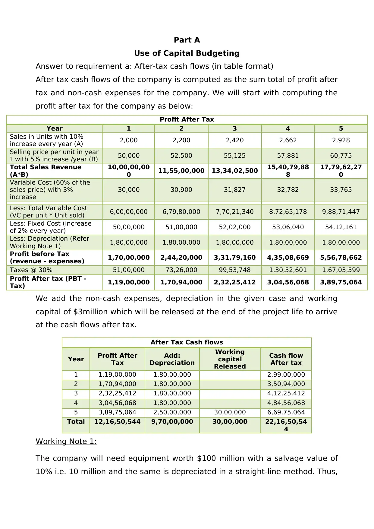
Answer to requirement a: After-tax cash flows (in table format)
After tax cash flows of the company is computed as the sum total of profit after
tax and non-cash expenses for the company. We will start with computing the
profit after tax for the company as below:
Profit After Tax
Year 1 2 3 4 5
Sales in Units with 10%
increase every year (A) 2,000 2,200 2,420 2,662 2,928
Selling price per unit in year
1 with 5% increase /year (B) 50,000 52,500 55,125 57,881 60,775
Total Sales Revenue
(A*B)
10,00,00,00
0 11,55,00,000 13,34,02,500 15,40,79,88
8
17,79,62,27
0
Variable Cost (60% of the
sales price) with 3%
increase
30,000 30,900 31,827 32,782 33,765
Less: Total Variable Cost
(VC per unit * Unit sold) 6,00,00,000 6,79,80,000 7,70,21,340 8,72,65,178 9,88,71,447
Less: Fixed Cost (increase
of 2% every year) 50,00,000 51,00,000 52,02,000 53,06,040 54,12,161
Less: Depreciation (Refer
Working Note 1) 1,80,00,000 1,80,00,000 1,80,00,000 1,80,00,000 1,80,00,000
Profit before Tax
(revenue - expenses) 1,70,00,000 2,44,20,000 3,31,79,160 4,35,08,669 5,56,78,662
Taxes @ 30% 51,00,000 73,26,000 99,53,748 1,30,52,601 1,67,03,599
Profit After tax (PBT -
Tax) 1,19,00,000 1,70,94,000 2,32,25,412 3,04,56,068 3,89,75,064
We add the non-cash expenses, depreciation in the given case and working
capital of $3million which will be released at the end of the project life to arrive
at the cash flows after tax.
After Tax Cash flows
Year Profit After
Tax
Add:
Depreciation
Working
capital
Released
Cash flow
After tax
1 1,19,00,000 1,80,00,000 2,99,00,000
2 1,70,94,000 1,80,00,000 3,50,94,000
3 2,32,25,412 1,80,00,000 4,12,25,412
4 3,04,56,068 1,80,00,000 4,84,56,068
5 3,89,75,064 2,50,00,000 30,00,000 6,69,75,064
Total 12,16,50,544 9,70,00,000 30,00,000 22,16,50,54
4
Working Note 1:
The company will need equipment worth $100 million with a salvage value of
10% i.e. 10 million and the same is depreciated in a straight-line method. Thus,

depreciation = $100 million - $10 million = $90 million/5 years = $1.8 million
or $1,800,000.
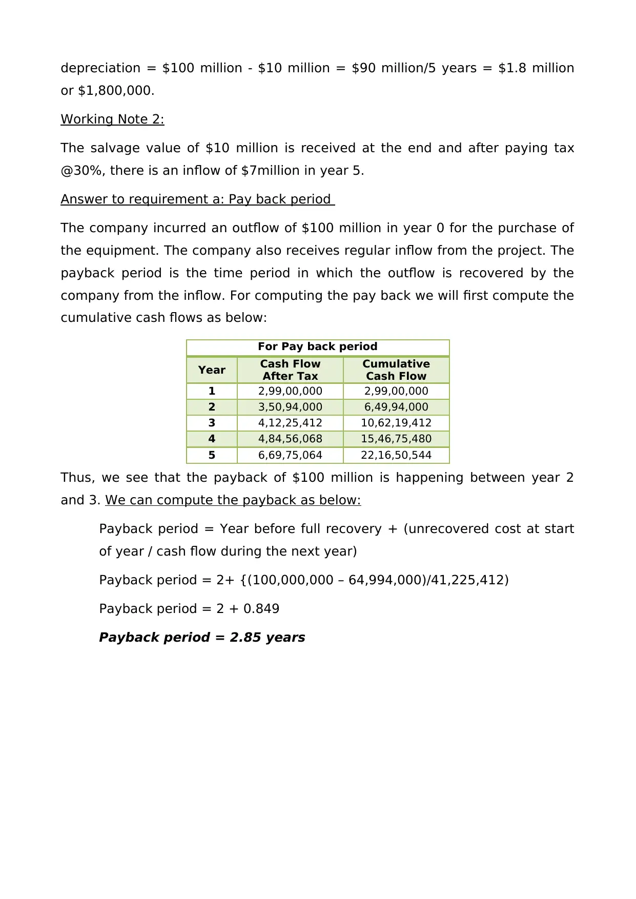
Working Note 2:
The salvage value of $10 million is received at the end and after paying tax
@30%, there is an inflow of $7million in year 5.
Answer to requirement a: Pay back period
The company incurred an outflow of $100 million in year 0 for the purchase of
the equipment. The company also receives regular inflow from the project. The
payback period is the time period in which the outflow is recovered by the
company from the inflow. For computing the pay back we will first compute the
cumulative cash flows as below:
For Pay back period
Year Cash Flow
After Tax
Cumulative
Cash Flow
1 2,99,00,000 2,99,00,000
2 3,50,94,000 6,49,94,000
3 4,12,25,412 10,62,19,412
4 4,84,56,068 15,46,75,480
5 6,69,75,064 22,16,50,544
Thus, we see that the payback of $100 million is happening between year 2
and 3. We can compute the payback as below:
Payback period = Year before full recovery + (unrecovered cost at start
of year / cash flow during the next year)
Payback period = 2+ {(100,000,000 – 64,994,000)/41,225,412)
Payback period = 2 + 0.849
Payback period = 2.85 years

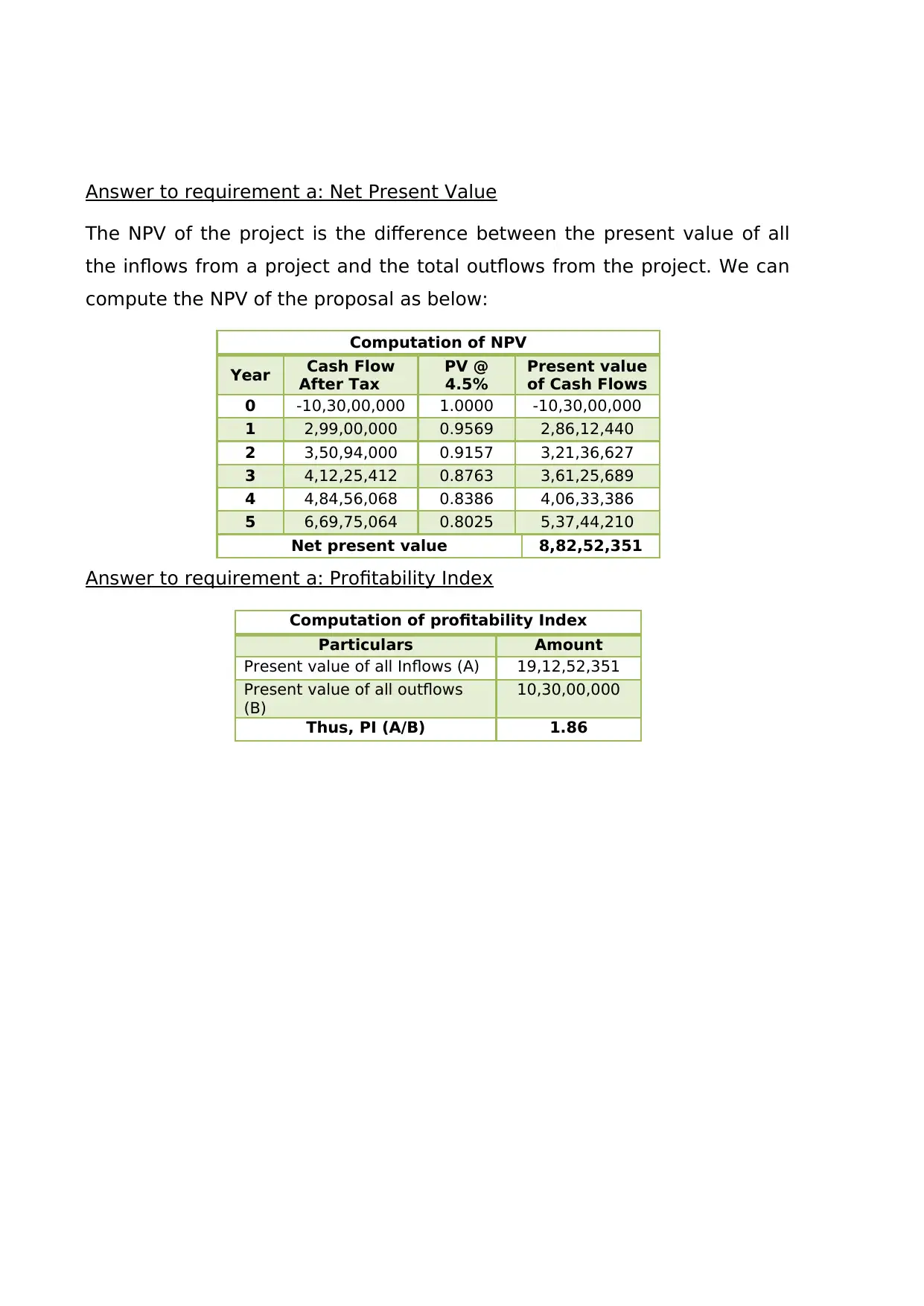
Answer to requirement a: Net Present Value
The NPV of the project is the difference between the present value of all
the inflows from a project and the total outflows from the project. We can
compute the NPV of the proposal as below:
Computation of NPV
Year Cash Flow
After Tax
PV @
4.5%
Present value
of Cash Flows
0 -10,30,00,000 1.0000 -10,30,00,000
1 2,99,00,000 0.9569 2,86,12,440
2 3,50,94,000 0.9157 3,21,36,627
3 4,12,25,412 0.8763 3,61,25,689
4 4,84,56,068 0.8386 4,06,33,386
5 6,69,75,064 0.8025 5,37,44,210
Net present value 8,82,52,351
Answer to requirement a: Profitability Index
Computation of profitability Index
Particulars Amount
Present value of all Inflows (A) 19,12,52,351
Present value of all outflows
(B)
10,30,00,000
Thus, PI (A/B) 1.86

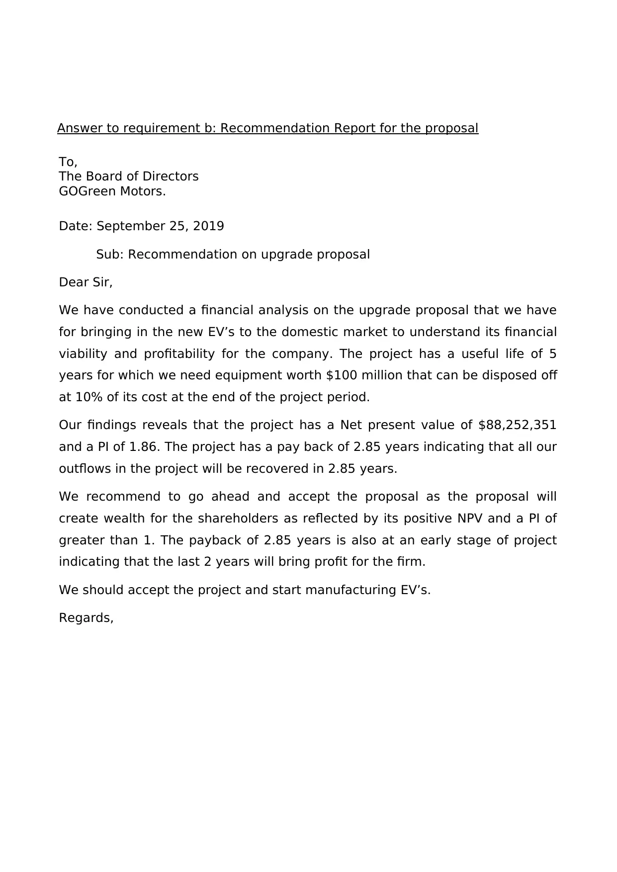
Answer to requirement b: Recommendation Report for the proposal
To,
The Board of Directors
GOGreen Motors.
Date: September 25, 2019
Sub: Recommendation on upgrade proposal
Dear Sir,
We have conducted a financial analysis on the upgrade proposal that we have
for bringing in the new EV’s to the domestic market to understand its financial
viability and profitability for the company. The project has a useful life of 5
years for which we need equipment worth $100 million that can be disposed off
at 10% of its cost at the end of the project period.
Our findings reveals that the project has a Net present value of $88,252,351
and a PI of 1.86. The project has a pay back of 2.85 years indicating that all our
outflows in the project will be recovered in 2.85 years.
We recommend to go ahead and accept the proposal as the proposal will
create wealth for the shareholders as reflected by its positive NPV and a PI of
greater than 1. The payback of 2.85 years is also at an early stage of project
indicating that the last 2 years will bring profit for the firm.
We should accept the project and start manufacturing EV’s.
Regards,

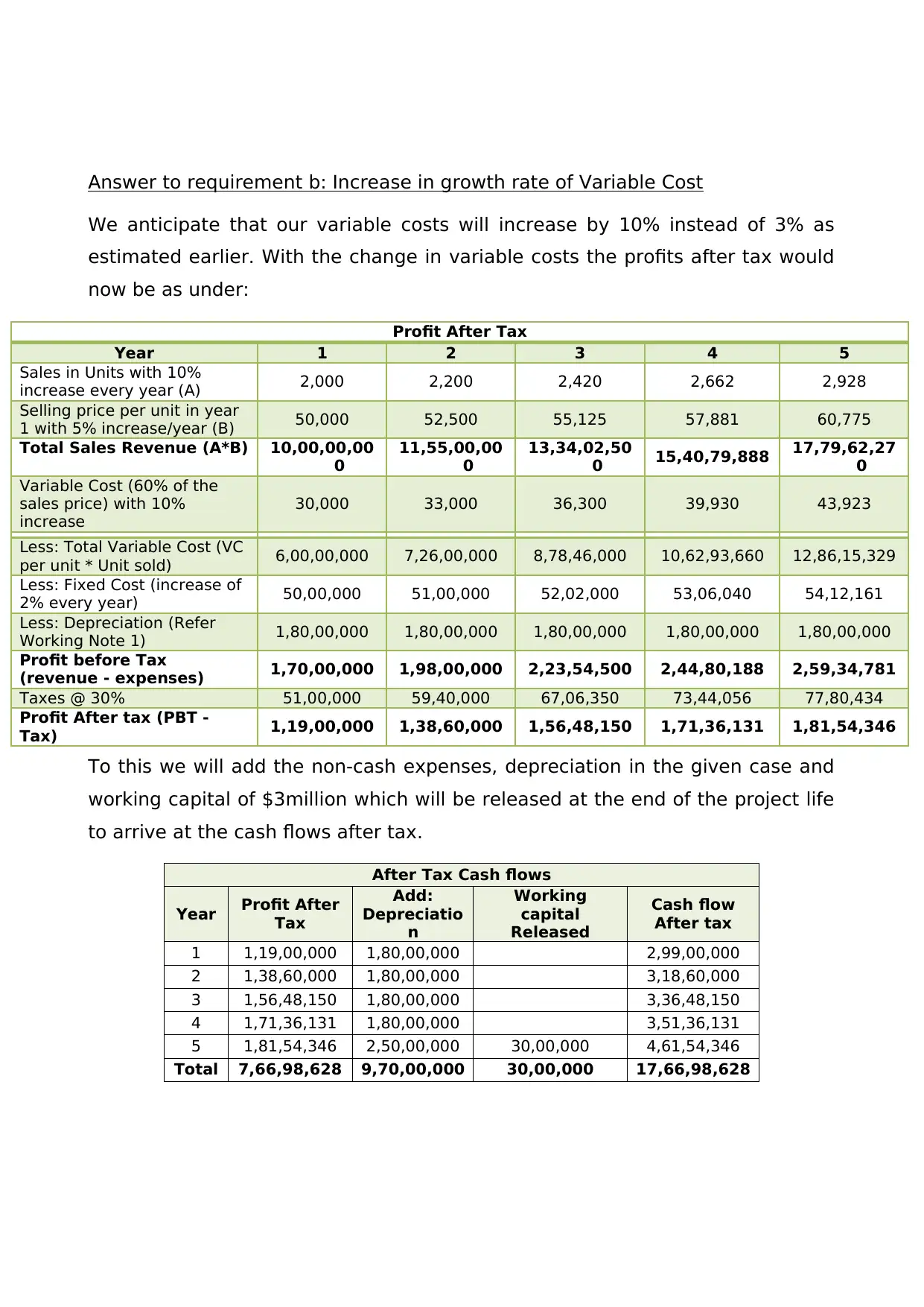
Answer to requirement b: Increase in growth rate of Variable Cost
We anticipate that our variable costs will increase by 10% instead of 3% as
estimated earlier. With the change in variable costs the profits after tax would
now be as under:
Profit After Tax
Year 1 2 3 4 5
Sales in Units with 10%
increase every year (A) 2,000 2,200 2,420 2,662 2,928
Selling price per unit in year
1 with 5% increase/year (B) 50,000 52,500 55,125 57,881 60,775
Total Sales Revenue (A*B) 10,00,00,00
0
11,55,00,00
0
13,34,02,50
0 15,40,79,888 17,79,62,27
0
Variable Cost (60% of the
sales price) with 10%
increase
30,000 33,000 36,300 39,930 43,923
Less: Total Variable Cost (VC
per unit * Unit sold) 6,00,00,000 7,26,00,000 8,78,46,000 10,62,93,660 12,86,15,329
Less: Fixed Cost (increase of
2% every year) 50,00,000 51,00,000 52,02,000 53,06,040 54,12,161
Less: Depreciation (Refer
Working Note 1) 1,80,00,000 1,80,00,000 1,80,00,000 1,80,00,000 1,80,00,000
Profit before Tax
(revenue - expenses) 1,70,00,000 1,98,00,000 2,23,54,500 2,44,80,188 2,59,34,781
Taxes @ 30% 51,00,000 59,40,000 67,06,350 73,44,056 77,80,434
Profit After tax (PBT -
Tax) 1,19,00,000 1,38,60,000 1,56,48,150 1,71,36,131 1,81,54,346
To this we will add the non-cash expenses, depreciation in the given case and
working capital of $3million which will be released at the end of the project life
to arrive at the cash flows after tax.
After Tax Cash flows
Year Profit After
Tax
Add:
Depreciatio
n
Working
capital
Released
Cash flow
After tax
1 1,19,00,000 1,80,00,000 2,99,00,000
2 1,38,60,000 1,80,00,000 3,18,60,000
3 1,56,48,150 1,80,00,000 3,36,48,150
4 1,71,36,131 1,80,00,000 3,51,36,131
5 1,81,54,346 2,50,00,000 30,00,000 4,61,54,346
Total 7,66,98,628 9,70,00,000 30,00,000 17,66,98,628

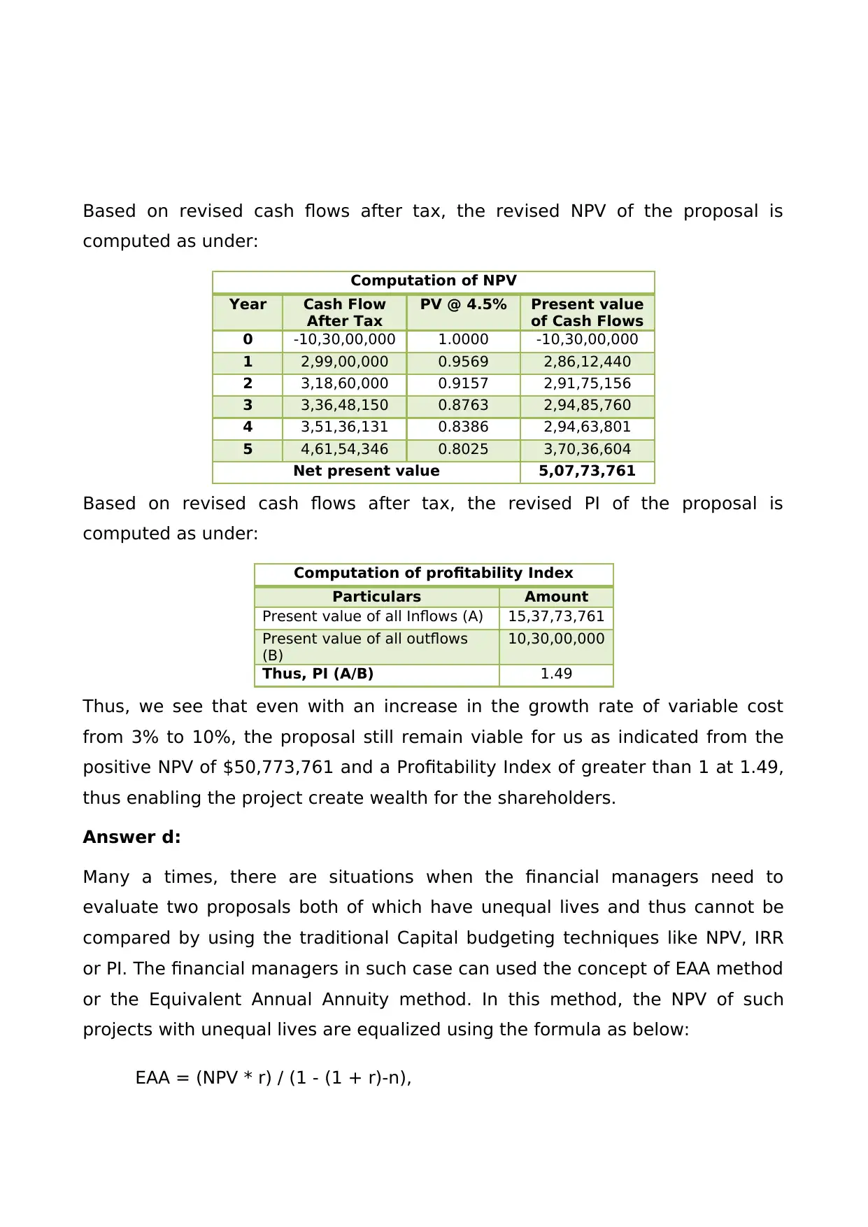
Based on revised cash flows after tax, the revised NPV of the proposal is
computed as under:
Computation of NPV
Year Cash Flow
After Tax
PV @ 4.5% Present value
of Cash Flows
0 -10,30,00,000 1.0000 -10,30,00,000
1 2,99,00,000 0.9569 2,86,12,440
2 3,18,60,000 0.9157 2,91,75,156
3 3,36,48,150 0.8763 2,94,85,760
4 3,51,36,131 0.8386 2,94,63,801
5 4,61,54,346 0.8025 3,70,36,604
Net present value 5,07,73,761
Based on revised cash flows after tax, the revised PI of the proposal is
computed as under:
Computation of profitability Index
Particulars Amount
Present value of all Inflows (A) 15,37,73,761
Present value of all outflows
(B)
10,30,00,000
Thus, PI (A/B) 1.49
Thus, we see that even with an increase in the growth rate of variable cost
from 3% to 10%, the proposal still remain viable for us as indicated from the
positive NPV of $50,773,761 and a Profitability Index of greater than 1 at 1.49,
thus enabling the project create wealth for the shareholders.
Answer d:
Many a times, there are situations when the financial managers need to
evaluate two proposals both of which have unequal lives and thus cannot be
compared by using the traditional Capital budgeting techniques like NPV, IRR
or PI. The financial managers in such case can used the concept of EAA method
or the Equivalent Annual Annuity method. In this method, the NPV of such
projects with unequal lives are equalized using the formula as below:
EAA = (NPV * r) / (1 - (1 + r)-n),

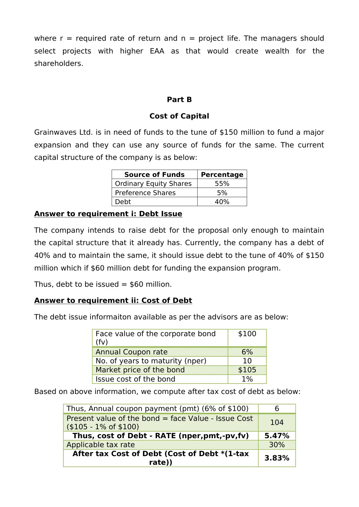
where r = required rate of return and n = project life. The managers should
select projects with higher EAA as that would create wealth for the
shareholders.
Part B
Cost of Capital
Grainwaves Ltd. is in need of funds to the tune of $150 million to fund a major
expansion and they can use any source of funds for the same. The current
capital structure of the company is as below:
Source of Funds Percentage
Ordinary Equity Shares 55%
Preference Shares 5%
Debt 40%
Answer to requirement i: Debt Issue
The company intends to raise debt for the proposal only enough to maintain
the capital structure that it already has. Currently, the company has a debt of
40% and to maintain the same, it should issue debt to the tune of 40% of $150
million which if $60 million debt for funding the expansion program.
Thus, debt to be issued = $60 million.
Answer to requirement ii: Cost of Debt
The debt issue informaiton available as per the advisors are as below:
Face value of the corporate bond
(fv)
$100
Annual Coupon rate 6%
No. of years to maturity (nper) 10
Market price of the bond $105
Issue cost of the bond 1%
Based on above information, we compute after tax cost of debt as below:
Thus, Annual coupon payment (pmt) (6% of $100) 6
Present value of the bond = face Value - Issue Cost
($105 - 1% of $100) 104
Thus, cost of Debt - RATE (nper,pmt,-pv,fv) 5.47%
Applicable tax rate 30%
After tax Cost of Debt (Cost of Debt *(1-tax
rate)) 3.83%

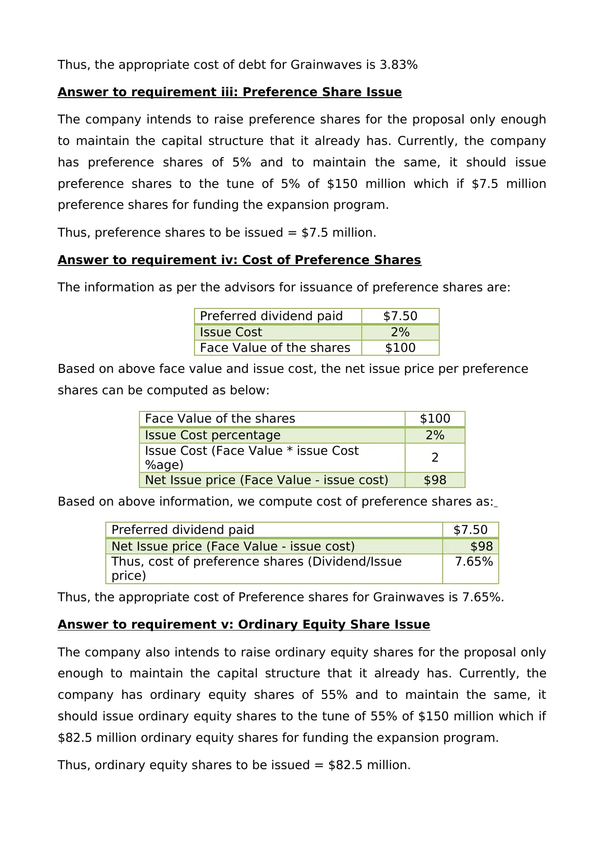
Thus, the appropriate cost of debt for Grainwaves is 3.83%
Answer to requirement iii: Preference Share Issue
The company intends to raise preference shares for the proposal only enough
to maintain the capital structure that it already has. Currently, the company
has preference shares of 5% and to maintain the same, it should issue
preference shares to the tune of 5% of $150 million which if $7.5 million
preference shares for funding the expansion program.
Thus, preference shares to be issued = $7.5 million.
Answer to requirement iv: Cost of Preference Shares
The information as per the advisors for issuance of preference shares are:
Preferred dividend paid $7.50
Issue Cost 2%
Face Value of the shares $100
Based on above face value and issue cost, the net issue price per preference
shares can be computed as below:
Face Value of the shares $100
Issue Cost percentage 2%
Issue Cost (Face Value * issue Cost
%age) 2
Net Issue price (Face Value - issue cost) $98
Based on above information, we compute cost of preference shares as:
Preferred dividend paid $7.50
Net Issue price (Face Value - issue cost) $98
Thus, cost of preference shares (Dividend/Issue
price)
7.65%
Thus, the appropriate cost of Preference shares for Grainwaves is 7.65%.
Answer to requirement v: Ordinary Equity Share Issue
The company also intends to raise ordinary equity shares for the proposal only
enough to maintain the capital structure that it already has. Currently, the
company has ordinary equity shares of 55% and to maintain the same, it
should issue ordinary equity shares to the tune of 55% of $150 million which if
$82.5 million ordinary equity shares for funding the expansion program.
Thus, ordinary equity shares to be issued = $82.5 million.

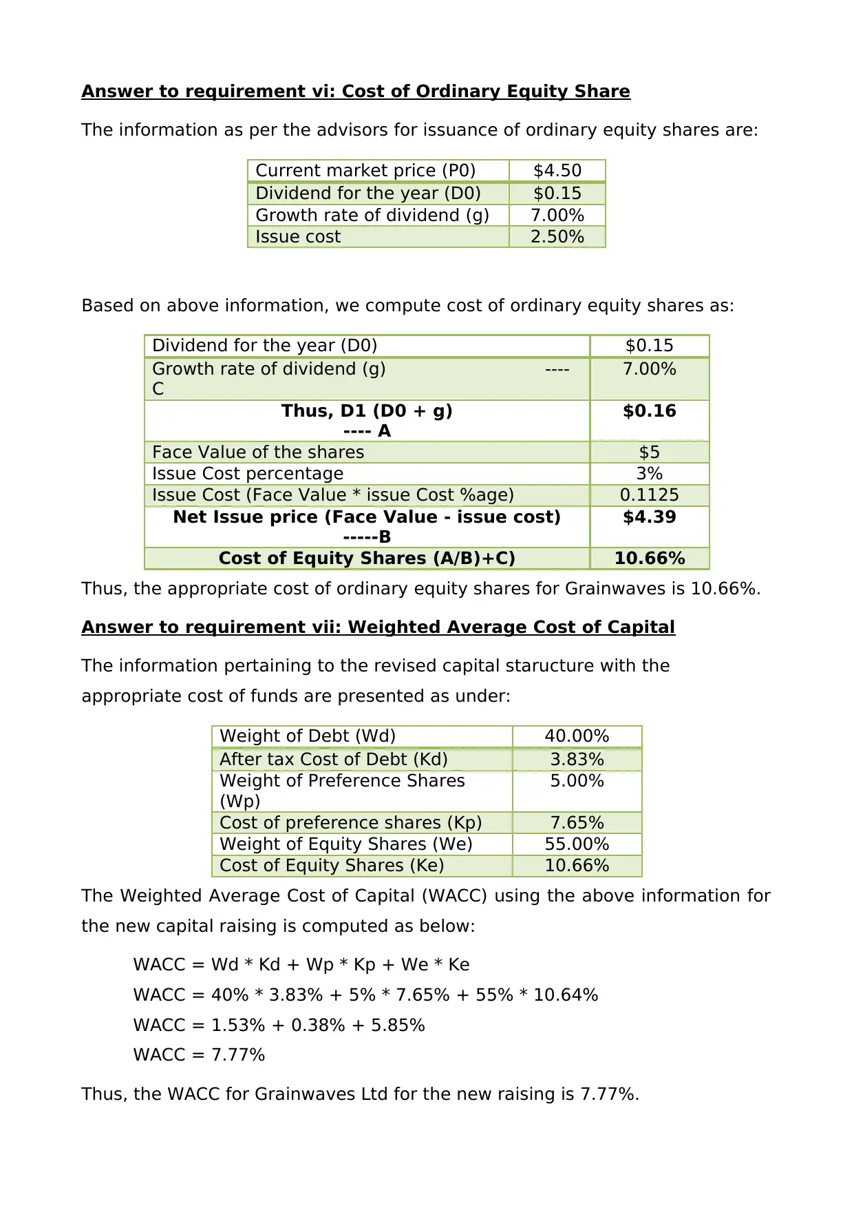
Answer to requirement vi: Cost of Ordinary Equity Share
The information as per the advisors for issuance of ordinary equity shares are:
Current market price (P0) $4.50
Dividend for the year (D0) $0.15
Growth rate of dividend (g) 7.00%
Issue cost 2.50%
Based on above information, we compute cost of ordinary equity shares as:
Dividend for the year (D0) $0.15
Growth rate of dividend (g) ----
C
7.00%
Thus, D1 (D0 + g)
---- A
$0.16
Face Value of the shares $5
Issue Cost percentage 3%
Issue Cost (Face Value * issue Cost %age) 0.1125
Net Issue price (Face Value - issue cost)
-----B
$4.39
Cost of Equity Shares (A/B)+C) 10.66%
Thus, the appropriate cost of ordinary equity shares for Grainwaves is 10.66%.
Answer to requirement vii: Weighted Average Cost of Capital
The information pertaining to the revised capital staructure with the
appropriate cost of funds are presented as under:
Weight of Debt (Wd) 40.00%
After tax Cost of Debt (Kd) 3.83%
Weight of Preference Shares
(Wp)
5.00%
Cost of preference shares (Kp) 7.65%
Weight of Equity Shares (We) 55.00%
Cost of Equity Shares (Ke) 10.66%
The Weighted Average Cost of Capital (WACC) using the above information for
the new capital raising is computed as below:
WACC = Wd * Kd + Wp * Kp + We * Ke
WACC = 40% * 3.83% + 5% * 7.65% + 55% * 10.64%
WACC = 1.53% + 0.38% + 5.85%
WACC = 7.77%
Thus, the WACC for Grainwaves Ltd for the new raising is 7.77%.

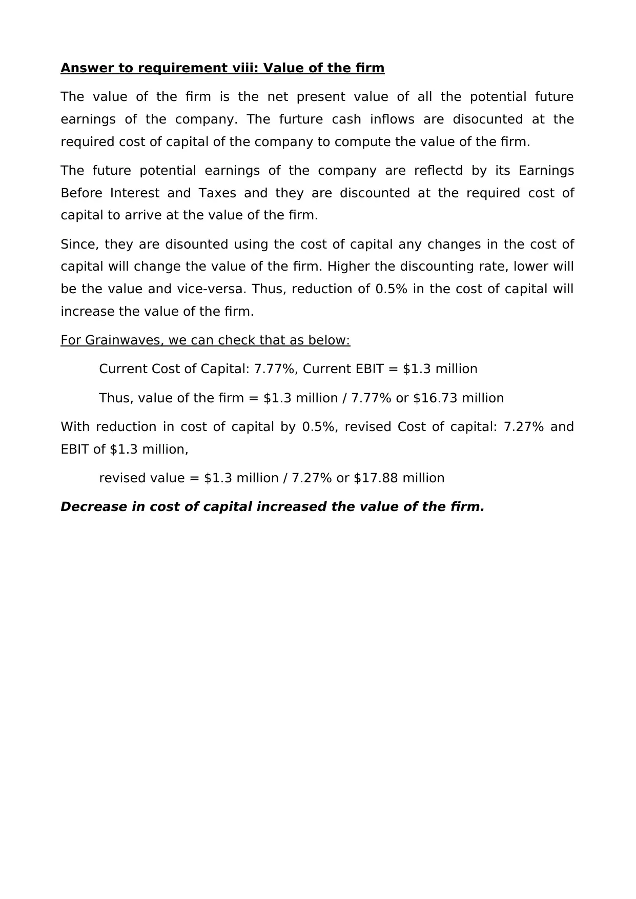
Answer to requirement viii: Value of the firm
The value of the firm is the net present value of all the potential future
earnings of the company. The furture cash inflows are disocunted at the
required cost of capital of the company to compute the value of the firm.
The future potential earnings of the company are reflectd by its Earnings
Before Interest and Taxes and they are discounted at the required cost of
capital to arrive at the value of the firm.
Since, they are disounted using the cost of capital any changes in the cost of
capital will change the value of the firm. Higher the discounting rate, lower will
be the value and vice-versa. Thus, reduction of 0.5% in the cost of capital will
increase the value of the firm.
For Grainwaves, we can check that as below:
Current Cost of Capital: 7.77%, Current EBIT = $1.3 million
Thus, value of the firm = $1.3 million / 7.77% or $16.73 million
With reduction in cost of capital by 0.5%, revised Cost of capital: 7.27% and
EBIT of $1.3 million,
revised value = $1.3 million / 7.27% or $17.88 million
Decrease in cost of capital increased the value of the firm.

References
Atrill, P.(2009). Financial management for decision makers, 5th edn., England:
FT Prentice Hall.
Block, S. (2019). Foundations of financial management. New York: McGraw-Hill.