Understanding Capital Market Line, Security Market Line, and CAPM

This report provides a detailed explanation of the Capital Market Line (CML), the Security Market Line (SML), and the Capital Asset Pricing Model (CAPM). It begins by outlining the assumptions of the CML, including homogeneous expectations and the market portfolio, and describes how investors combine the market portfolio with a risk-free asset to form efficient portfolios. The report then explains the relationship between risk and return on the CML, and the formula used to calculate expected returns. The report then transitions to the SML, which illustrates the relationship between expected return and beta for all securities and portfolios, whether efficient or inefficient. It differentiates between systematic and unsystematic risk, emphasizing the importance of beta as a measure of systematic risk. The report also provides formulas for calculating expected return based on beta and the market risk premium. Finally, the report contrasts the CML and SML, and explains how the CAPM can be used for security valuation, including identifying underpriced and overpriced securities based on their position relative to the SML.

THE CAPITAL MARKET LINE
All investors are assumed to have identical (homogeneous) expectations. Hence, all of
them will face the same efficient frontier depicted in Fig. Every investor will seek to
combine the same risky portfolio B with different levels of lending or borrowing according to
his desired level of risk. Because all investors hold the same risky portfolio, then it will
include all risky securities in the market. This portfolio of all risky securities is referred to as
the market portfolio M. Each security will be held in the proportion which the market value
of the security bears to the total market value of all risky securities in the market. All
investors will hold combinations of only two assets, the market portfolio and a riskless
security.
All these combinations will lie along the straight line representing the efficient
frontier. This line formed by the action of all investors mixing the market portfolio with the
risk free asset is known as the capital market line (CML). All efficient portfolios of all
investors will lie along this capital market line.
The relationship between the return and risk of any efficient portfolio on the capital
market line can be expressed in the form of the following equation.
Re = Rf + [ Re – Rf] σe
σm
Where the subscript e denotes an efficient portfolio.
The risk free return Rf represents the reward for waiting. It is, in other words, the
price of time. The term [(Rm – Rf/σ m] represents the price of risk or risk premium, i.e. the
excess return earned per unit of risk or standard deviation. It measures the additional return
for an additional unit of risk. When the risk of the efficient portfolio, σ e , is multiplied with
this term, we get the risk premium available for the particular efficient portfolio under
consideration.
Thus, the expected return on an efficient portfolio is :
(Expected return) = (Price of time) + (Price of risk) (Amount of risk)
The CML provides a risk return relationship and a measure of risk for efficient
portfolios. The appropriate measure of risk for an efficient portfolio is the standard deviation
of return of the portfolio. There is a linear relationship between the risk as measured by the
standard deviation and the expected return for these efficient portfolios.

THE SECURITY MARKET LINE
The CML shows the risk – return relationship for all efficient portfolios. They would
all lie along the capital market line. All portfolios other than the efficient ones will lie below
the capital market line. The CML does not describe the risk – return relationship of inefficient
portfolios or of individual securities. The capital asset pricing model specifies the relationship
between expected return and risk for all securities and all portfolios, whether efficient or
inefficient.
We have seen earlier that the total risk of a security as measured by standard deviation
is compared of two components: systematic risk and unsystematic risk or diversifiable risk.
As investment is diversified and more and more securities are added to a portfolio, the
unsystematic risk is reduced. For a very well diversified portfolio, unsystematic risk trends to
become zero and the only relevant risk is systematic risk measured by beta (β). Hence, it is
argued that the correct measure of a security‘s risk is beta.
It follows that the expected return of a security or of a portfolio should be related to
the risk of that security or portfolios as measured by β. Beta is a measure of the security‘s
sensitivity to change in market return. Beta value greater than one indicates higher sensitivity
to market changes, whereas beta value less than one indicates lower sensitivity to market
changes. A β value of one indicates that the security moves at the same rate and in the same
direction as the market. Thus, the β of the market may be taken as one.
The relationship between expected return and β of a security can be determined
graphically. Let us consider and XY graph where expected returns are plotted on the Y axis
and beta coefficients are plotted on the X axis. A risk free asset has an expected return
equivalent to Rf and beta coefficient of zero. The market portfolio M has a beta coefficient of
one and expected return equivalent R m. A straight line joining these two points is known as
the security market line (SML). This is illustrated in Fig. 1
The security market line provides the relationship between the expected return and
beta of a security or portfolio. This relationship can be expressed in the form of the following
equation:
Rm – Rf + βi (Rm - Rf )
A part of the return on any security or portfolio is a reward for bearing risk and the
rest is the reward for waiting, representing the time value of money. The risk free rate, R f
(which is earned by a security which has no risk) is the reward for waiting. The reward for
bearing risk is the risk premium. The risk premium of a security is directly proportional to the
risk as measured by β. The risk premium of a security is calculated as the product of beta and
the risk premium of the market which is the excess of expected market return over the risk
free return, that is, [Rm - Rf ].

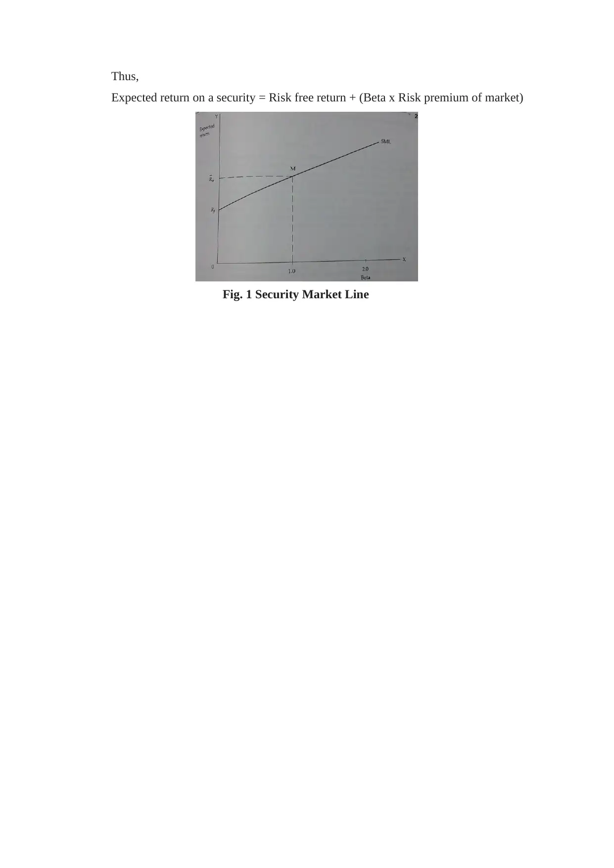
Thus,
Expected return on a security = Risk free return + (Beta x Risk premium of market)
Fig. 1 Security Market Line

CAPM
The relationship between risk and return established by the security market line in
known as the capital asset pricing model. It is basically a simple linear relationship. The
higher the value of beta, higher would be the risk of the security and therefore, larger would
be the return expected by the investors. In other words, all securities are expected to yield
returns commensurate with their riskiness as measured by β. This relationship is valid not
only for individual securities, but it also valid for all portfolios whether efficient or
inefficient.
The expected return on any security or portfolio can be determined from the CAPM
formula if we know the beta of that security or portfolio. To illustrate the application of the
CAPM, let us consider a simple example. There are two securities P and Q having values of
beta as 0.7 and 1.6 respectively. The risk free rate is assumed to be 6 per cent and the market
return is expected to be 15 per cent, thus providing a market risk premium of 9 per cent (i.e.
Rm - Rf ).
The expected return on security P may be worked out as shown below:
Rm = Rf + βi [Rm - Rf )
= 6 + 0.7 (15 – 6)
= 6 + 6.3 = 12.3 per cent
The expected return on security Q is
Rm = 6 + 1.6 (15 – 6)
= 6 + 14.4
= 20.4 per cent
Security P with a β of 0.7 has an expected return of 12.3 per cent whereas security Q
with a higher beta of 1.6 has a higher expected return of 20.4 per cent.
CAPM represents one of the most important discoveries in the field of fiancé. It
describes the expected return for all assets and portfolios of assets in the economy. The
difference in the expected returns of any two assets can be related to the difference in their
betas. The model postulates that systematic risk is the only important ingredient in
determining expected return. As investors can eliminate all unsystematic risk through
diversification, they can be expected to be rewarded only for bearing systematic risk. Thus,
the relevant risk of an asset is its systematic risk and not the total risk.

SML AND CML
It is necessary to contrast SML with CML. Both postulate a linear (straight line)
relationship between risk and return. In CML the risk is defined as total risk and is measured
by standard deviation, while in SML the risk is defined as systematic risk and is measured by
β. Capital market line is valid only for efficient portfolios while security market line is valid
for all portfolios and all individual securities as well. CML is the basis of the capital market
theory while SML is the basis of the capital asset pricing model.
PRICING OF SECURITIES WITH CAPM
The capital asset pricing model can also be used for evaluating the pricing of
securities. The CAPM provides a framework for assessing whether a security is underpriced,
overpriced or correctly priced. According to CAPM, each security is expected to provide a
return commensurate with its level of risk. A security may be offering more returns than the
expected return, making it more attractive. On the contrary, another security may be offering
less return than the expected return, making it less attractive.
The expected return on a security can be calculating using the CAPM formula. Let us
designate it as the theoretical return. The real rate of return estimated to be realsied from
investing in a security can be calculated by the following formula.
Ri = (P1 – P0) + D1
P0

Where
P0 = Current market price.
P1 = Estimated market price after one year
D1 = Anticipated dividend for the year.
This may be designated as the estimated return.
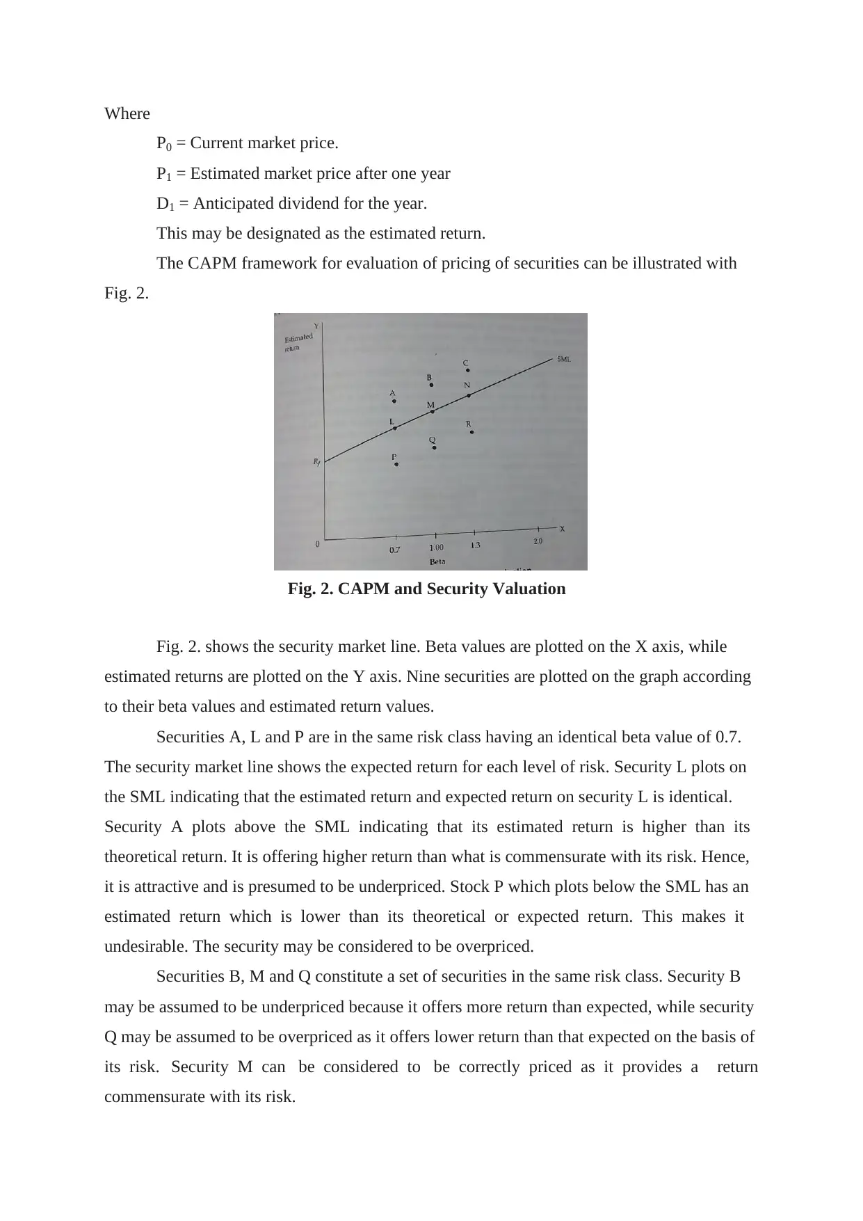
The CAPM framework for evaluation of pricing of securities can be illustrated with
Fig. 2.
Fig. 2. CAPM and Security Valuation
Fig. 2. shows the security market line. Beta values are plotted on the X axis, while
estimated returns are plotted on the Y axis. Nine securities are plotted on the graph according
to their beta values and estimated return values.
Securities A, L and P are in the same risk class having an identical beta value of 0.7.
The security market line shows the expected return for each level of risk. Security L plots on
the SML indicating that the estimated return and expected return on security L is identical.
Security A plots above the SML indicating that its estimated return is higher than its
theoretical return. It is offering higher return than what is commensurate with its risk. Hence,
it is attractive and is presumed to be underpriced. Stock P which plots below the SML has an
estimated return which is lower than its theoretical or expected return. This makes it
undesirable. The security may be considered to be overpriced.
Securities B, M and Q constitute a set of securities in the same risk class. Security B
may be assumed to be underpriced because it offers more return than expected, while security
Q may be assumed to be overpriced as it offers lower return than that expected on the basis of
its risk. Security M can be considered to be correctly priced as it provides a return
commensurate with its risk.

Securities C,N and R constitute another set of securities belonging to the same risk
class, each having a beta value of 1.3. It can be seen that security C is underpriced, security R
is overpriced and security N is correctly priced.
Thus, in the context of the security market line, securities that plot above the line
presumably are underpriced because they offer a higher return than that expected from
securities with same risk. On the other hand, a security is presumably overpriced if it plots
below the SML because it is estimated to provide a lower return than that expected from
securities in the same risk class. Securities which plot on SML are assumed to be
appropriately priced in the context of CAPM. These securities are offering returns in line
with their riskiness.
Securities plotting off the security market line would be evidence of mispricing in the
market place. CAPM can be used to identify and overpriced securities. If the expected return
on a security calculated according to CAPM is lower than the actual or estimated return
offered by that security, the security will be considered to be underpriced. On the contrary, a
security will be considered to be overpriced when the expected return on the security
according to CAPM formulation is higher than the actual return offered by the security.
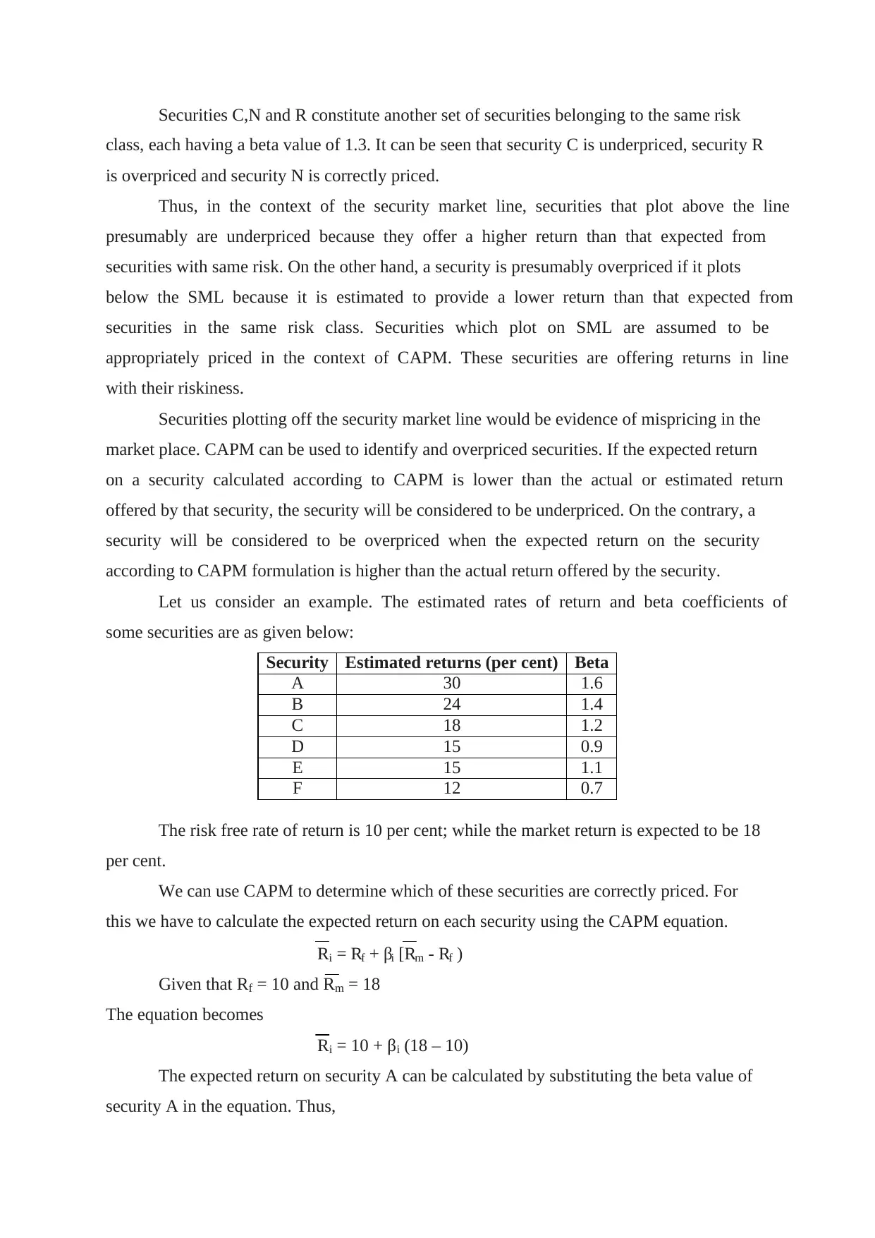
Let us consider an example. The estimated rates of return and beta coefficients of
some securities are as given below:
Security Estimated returns (per cent) Beta
A 30 1.6
B 24 1.4
C 18 1.2
D 15 0.9
E 15 1.1
F 12 0.7
The risk free rate of return is 10 per cent; while the market return is expected to be 18
per cent.
We can use CAPM to determine which of these securities are correctly priced. For
this we have to calculate the expected return on each security using the CAPM equation.
Ri = Rf + βi [Rm - Rf )
Given that Rf = 10 and Rm = 18
The equation becomes
Ri = 10 + βi (18 – 10)
The expected return on security A can be calculated by substituting the beta value of
security A in the equation. Thus,

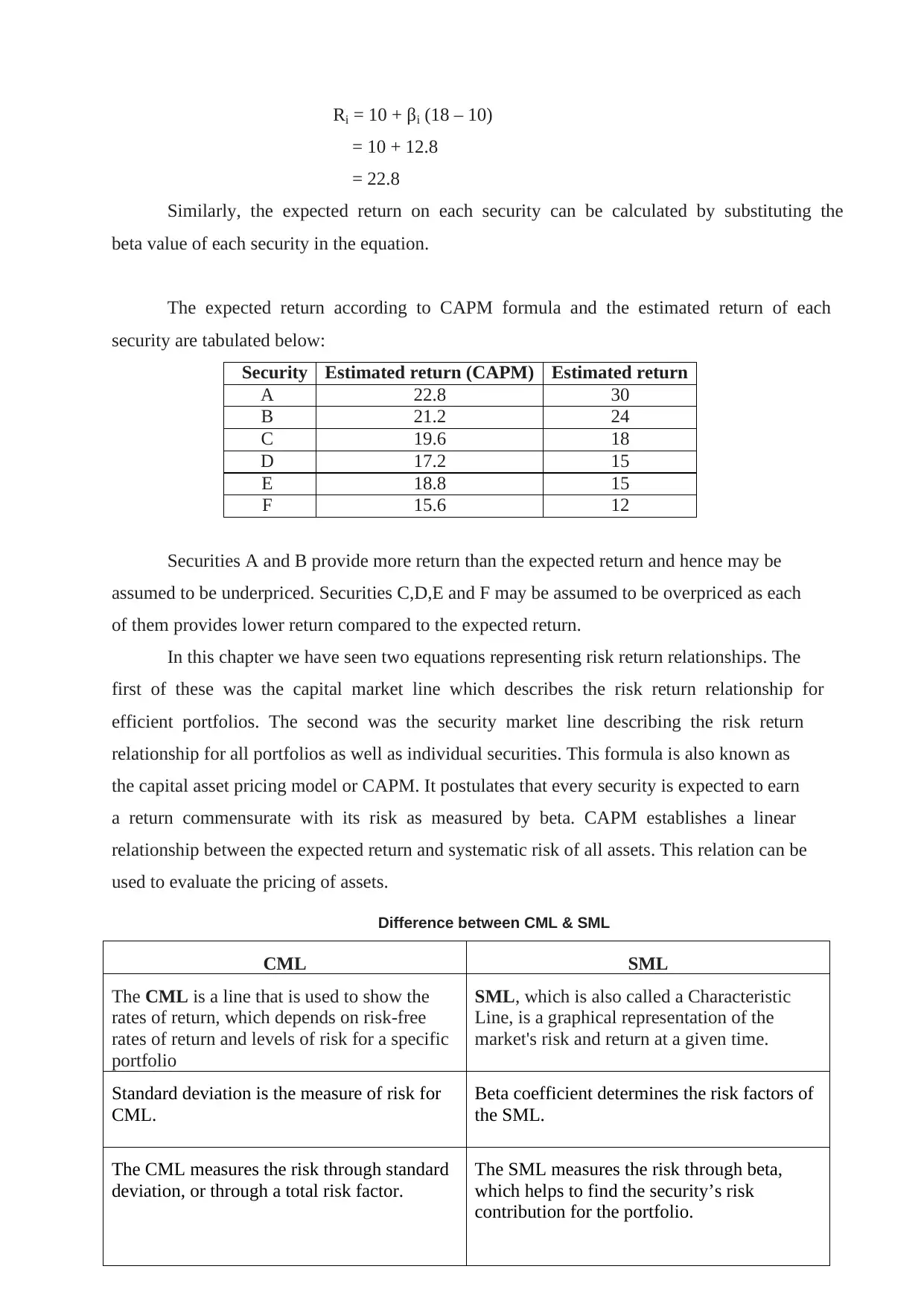
Ri = 10 + βi (18 – 10)
= 10 + 12.8
= 22.8
Similarly, the expected return on each security can be calculated by substituting the
beta value of each security in the equation.
The expected return according to CAPM formula and the estimated return of each
security are tabulated below:
Security Estimated return (CAPM) Estimated return
A 22.8 30
B 21.2 24
C 19.6 18
D 17.2 15
E 18.8 15
F 15.6 12
Securities A and B provide more return than the expected return and hence may be
assumed to be underpriced. Securities C,D,E and F may be assumed to be overpriced as each
of them provides lower return compared to the expected return.
In this chapter we have seen two equations representing risk return relationships. The
first of these was the capital market line which describes the risk return relationship for
efficient portfolios. The second was the security market line describing the risk return
relationship for all portfolios as well as individual securities. This formula is also known as
the capital asset pricing model or CAPM. It postulates that every security is expected to earn
a return commensurate with its risk as measured by beta. CAPM establishes a linear
relationship between the expected return and systematic risk of all assets. This relation can be
used to evaluate the pricing of assets.
Difference between CML & SML
CML SML
The CML is a line that is used to show the
rates of return, which depends on risk-free
rates of return and levels of risk for a specific
portfolio
SML, which is also called a Characteristic
Line, is a graphical representation of the
market's risk and return at a given time.
Standard deviation is the measure of risk for
CML.
Beta coefficient determines the risk factors of
the SML.
The CML measures the risk through standard
deviation, or through a total risk factor.
The SML measures the risk through beta,
which helps to find the security’s risk
contribution for the portfolio.

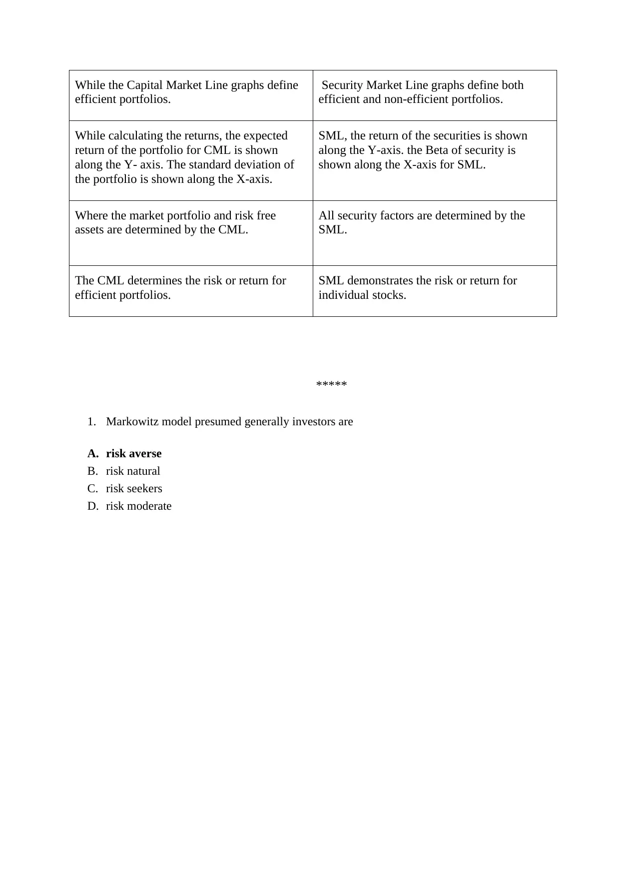
While the Capital Market Line graphs define
efficient portfolios.
Security Market Line graphs define both
efficient and non-efficient portfolios.
While calculating the returns, the expected
return of the portfolio for CML is shown
along the Y- axis. The standard deviation of
the portfolio is shown along the X-axis.
SML, the return of the securities is shown
along the Y-axis. the Beta of security is
shown along the X-axis for SML.
Where the market portfolio and risk free
assets are determined by the CML.
All security factors are determined by the
SML.
The CML determines the risk or return for
efficient portfolios.
SML demonstrates the risk or return for
individual stocks.
*****
1. Markowitz model presumed generally investors are
A. risk averse
B. risk natural
C. risk seekers
D. risk moderate