Car Insurance Fraud: Claims Prediction and Data Analysis Project
VerifiedAdded on 2023/02/01
|19
|4219
|73
Project
AI Summary
This project investigates car insurance fraud using a dataset of 1000 claimants. The study examines the relationship between individual claims (injury, property, vehicle) and total claim amounts. It explores the use of clustering, classification, and linear regression models to predict total claims based on attributes like age, policy deductibles, and premiums. The analysis includes correlation coefficients and visualizations using Tableau and R, revealing insights into claim trends. The project aims to assist insurance companies in making informed decisions about reserving, premium calculations, and policy deductibles, as well as identifying potential fraud. The findings highlight the importance of understanding the relationships between various claim types and their impact on overall claim amounts, with the goal of developing models to predict total claims and detect anomalies indicative of fraudulent activities. The project's methodology includes data preparation, model generation, and testing, with an emphasis on linear regression for prediction.
CAR INSURANCE FRAUD
1
CAR INSURANCE FRAUD
Name of institution:
Name of student:
Date:
Word count: 2157
1
CAR INSURANCE FRAUD
Name of institution:
Name of student:
Date:
Word count: 2157
Paraphrase This Document
Need a fresh take? Get an instant paraphrase of this document with our AI Paraphraser
CAR INSURANCE FRAUD
2
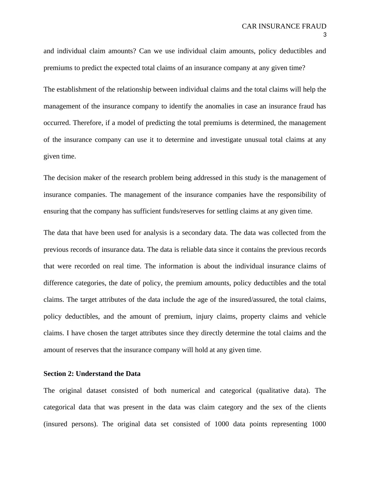
Section 1: The Problem
The amount the client of insurance companies (insured/assured) pay in order to be compensated
in the event of risk is known as the premium. Therefore, the amount of premium is equivalent to
the cost of getting an insurance cover or policy. An insurance cover or an insurance policy is the
contract binding the insured/assured and the insurance company. An insurance policy usually
comes with policy deductibles (Valles-Barjas & Fernando, 2015).
. A policy deductible is the amount of money that is being deducted from the premium for the
purpose of policy administrations. All these factors influences the total claim amounts as well as
the amount of individual claims.
An insurance claim that has been made in contrary to the agreements in the contract is an
insurance fraud. A fraud in insurance may result from numerous sources. The major cause of
insurance fraud is the collision between the insurance officers and the insured person. When an
insurance fraud occurs, the insurance company may experience a loss or reduction in the profits.
An insurance fraud may also result into increase in the total claims that the insurance pays.
Given the total claim amount, the individual claim amounts, the premiums and the policy
deductibles, an insurance company has a problem of maintaining sufficient amount of money
that can be used to settle the claims at any given time. The practice of maintaining sufficient
amount of money for insurance operations and claim compensations is known as reserving. The
problem that this study addresses is to investigate the relationship between individual claims and
the total claim amounts. The establishment of the relationship will help the insurance companies
to in making informed decisions about reserving, premium calculations and policy deductibles.
Therefore, the research question is: Can we establish the relationship between the total claims
2
Section 1: The Problem
The amount the client of insurance companies (insured/assured) pay in order to be compensated
in the event of risk is known as the premium. Therefore, the amount of premium is equivalent to
the cost of getting an insurance cover or policy. An insurance cover or an insurance policy is the
contract binding the insured/assured and the insurance company. An insurance policy usually
comes with policy deductibles (Valles-Barjas & Fernando, 2015).
. A policy deductible is the amount of money that is being deducted from the premium for the
purpose of policy administrations. All these factors influences the total claim amounts as well as
the amount of individual claims.
An insurance claim that has been made in contrary to the agreements in the contract is an
insurance fraud. A fraud in insurance may result from numerous sources. The major cause of
insurance fraud is the collision between the insurance officers and the insured person. When an
insurance fraud occurs, the insurance company may experience a loss or reduction in the profits.
An insurance fraud may also result into increase in the total claims that the insurance pays.
Given the total claim amount, the individual claim amounts, the premiums and the policy
deductibles, an insurance company has a problem of maintaining sufficient amount of money
that can be used to settle the claims at any given time. The practice of maintaining sufficient
amount of money for insurance operations and claim compensations is known as reserving. The
problem that this study addresses is to investigate the relationship between individual claims and
the total claim amounts. The establishment of the relationship will help the insurance companies
to in making informed decisions about reserving, premium calculations and policy deductibles.
Therefore, the research question is: Can we establish the relationship between the total claims
CAR INSURANCE FRAUD
3
and individual claim amounts? Can we use individual claim amounts, policy deductibles and
premiums to predict the expected total claims of an insurance company at any given time?
The establishment of the relationship between individual claims and the total claims will help the
management of the insurance company to identify the anomalies in case an insurance fraud has
occurred. Therefore, if a model of predicting the total premiums is determined, the management
of the insurance company can use it to determine and investigate unusual total claims at any
given time.
The decision maker of the research problem being addressed in this study is the management of
insurance companies. The management of the insurance companies have the responsibility of
ensuring that the company has sufficient funds/reserves for settling claims at any given time.
The data that have been used for analysis is a secondary data. The data was collected from the
previous records of insurance data. The data is reliable data since it contains the previous records
that were recorded on real time. The information is about the individual insurance claims of
difference categories, the date of policy, the premium amounts, policy deductibles and the total
claims. The target attributes of the data include the age of the insured/assured, the total claims,
policy deductibles, and the amount of premium, injury claims, property claims and vehicle
claims. I have chosen the target attributes since they directly determine the total claims and the
amount of reserves that the insurance company will hold at any given time.
Section 2: Understand the Data
The original dataset consisted of both numerical and categorical (qualitative data). The
categorical data that was present in the data was claim category and the sex of the clients
(insured persons). The original data set consisted of 1000 data points representing 1000
⊘ This is a preview!⊘
Do you want full access?
Subscribe today to unlock all pages.
Trusted by 1+ million students worldwide
CAR INSURANCE FRAUD
4
claimants during the period. The sample data that have been used for analysis consists of 8
attributes: The age of the insured, the amount of policy deductible, the amount of injury claims,
the amount of property claims, the amount vehicle claims, the premium and the amount of total
claims. The eight attributes were the most relevant attributes for this study.
The amount of vehicle claim, the amount of property claims and the amount of injury claims are
relevant for this study because they represents individual claims (An Creemers, et al., 2012). Total
claims amount is relevant because it represents the pool of all claims that an insurance company
pays to the insured. Policy deductible is relevant to this study because it directly affects the value
of total claims as well as the amount of reserves the insurance company will pay to the insured.
The eight attributes are all quantitative in nature. Similarly, the eight attributes are all numerical
in nature and can be quantified in terms of numbers.
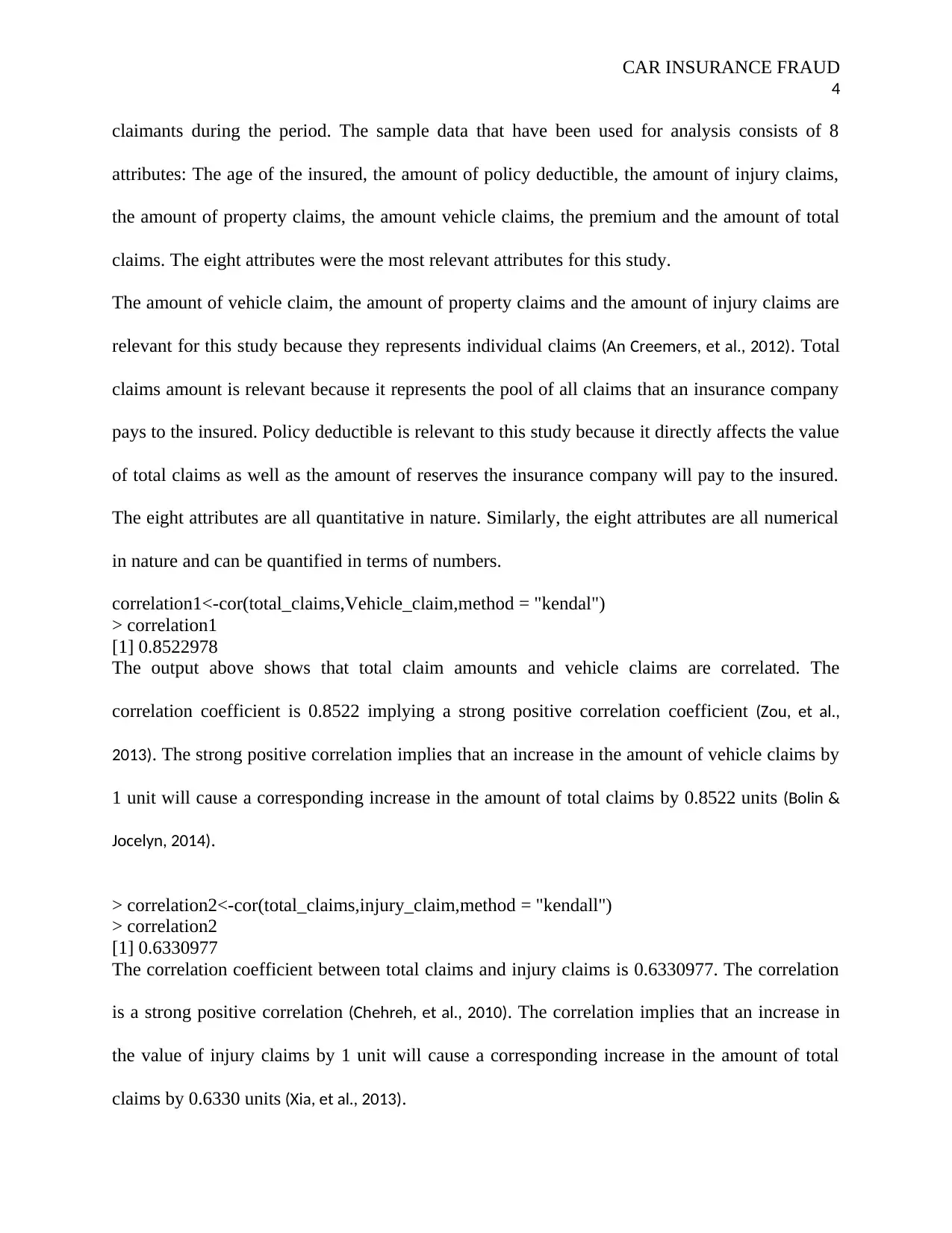
correlation1<-cor(total_claims,Vehicle_claim,method = "kendal")
> correlation1
[1] 0.8522978
The output above shows that total claim amounts and vehicle claims are correlated. The
correlation coefficient is 0.8522 implying a strong positive correlation coefficient (Zou, et al.,
2013). The strong positive correlation implies that an increase in the amount of vehicle claims by
1 unit will cause a corresponding increase in the amount of total claims by 0.8522 units (Bolin &
Jocelyn, 2014).
> correlation2<-cor(total_claims,injury_claim,method = "kendall")
> correlation2
[1] 0.6330977
The correlation coefficient between total claims and injury claims is 0.6330977. The correlation
is a strong positive correlation (Chehreh, et al., 2010). The correlation implies that an increase in
the value of injury claims by 1 unit will cause a corresponding increase in the amount of total
claims by 0.6330 units (Xia, et al., 2013).
4
claimants during the period. The sample data that have been used for analysis consists of 8
attributes: The age of the insured, the amount of policy deductible, the amount of injury claims,
the amount of property claims, the amount vehicle claims, the premium and the amount of total
claims. The eight attributes were the most relevant attributes for this study.
The amount of vehicle claim, the amount of property claims and the amount of injury claims are
relevant for this study because they represents individual claims (An Creemers, et al., 2012). Total
claims amount is relevant because it represents the pool of all claims that an insurance company
pays to the insured. Policy deductible is relevant to this study because it directly affects the value
of total claims as well as the amount of reserves the insurance company will pay to the insured.
The eight attributes are all quantitative in nature. Similarly, the eight attributes are all numerical
in nature and can be quantified in terms of numbers.
correlation1<-cor(total_claims,Vehicle_claim,method = "kendal")
> correlation1
[1] 0.8522978
The output above shows that total claim amounts and vehicle claims are correlated. The
correlation coefficient is 0.8522 implying a strong positive correlation coefficient (Zou, et al.,
2013). The strong positive correlation implies that an increase in the amount of vehicle claims by
1 unit will cause a corresponding increase in the amount of total claims by 0.8522 units (Bolin &
Jocelyn, 2014).
> correlation2<-cor(total_claims,injury_claim,method = "kendall")
> correlation2
[1] 0.6330977
The correlation coefficient between total claims and injury claims is 0.6330977. The correlation
is a strong positive correlation (Chehreh, et al., 2010). The correlation implies that an increase in
the value of injury claims by 1 unit will cause a corresponding increase in the amount of total
claims by 0.6330 units (Xia, et al., 2013).
Paraphrase This Document
Need a fresh take? Get an instant paraphrase of this document with our AI Paraphraser
CAR INSURANCE FRAUD
5
> correlation3<-cor(total_claims,property_claim)
> correlation3
[1] 0.8106865
The correlation coefficient between property claims and the total claims is 0.8106865. The
correlation coefficient is a strong positive correlation coefficient (Federico, et al., 2009). The
correlation coefficient implies that an increase in the value of total claims by 1 will cause a
corresponding increase in the value of property claims by 0.8106865 (Valles-Barjas & Fernando,
2015).
> correlation4<-cor(total_claims,age, method = "kendall")
> correlation4
[1] 0.04370292
The above output implies that the correlation coefficient between the amount of total claims and
the age of an insured is 0.04370 (Jieli, et al., 2012). The correlation is a weak correlation
coefficient. The correlation implies that an increase in the value of the age of an insured by 1 unit
will cause a corresponding increase in the value of total claims by 0.04370 units (Sungduk, et al.,
2011).
> correlation5<-cor(total_claims,Policy_Deductible, method = "kendall")
> correlation5
[1] 0.01577333
The correlation coefficient between the amount of policy deductible and the amount of total
claims is 0.01577. The correlation is a weak positive correlation (Jieli, et al., 2012). The correlation
implies that an increase in the value of policy deductible by 1 unit will cause a corresponding
increase in the value of total claims by 0.0157733 (Richard, 2009).
> correlation6<-cor(total_claims,annual_premium,method="kendall")
> correlation6
CAR INSURANCE FRAUD
6
[1] 0.0002062721
The correlation coefficient between the amount of annual premiums and the amount of total
claims is 0.0002062721 (Levin & Paul, 2016). The correlation is a weak negative correlation. The
correlation coefficient implies that an increase in the value of annual premiums by 1 unit will
cause a corresponding increase in the value of total premiums by 0.0002062721 (Revan, 2009).
The Different types of Tableau visualization
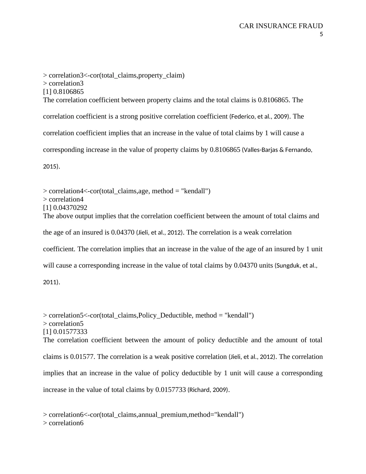
The graphs below shows visualization of the attributes in Tableau. The first graph is the graph of
property claims against the age of insured (Qihua & Gregg, 2011). The line graph provides the
trend of property claims. The trend reveals that the amount of property claims decreases with an
increase in the age of the insured.
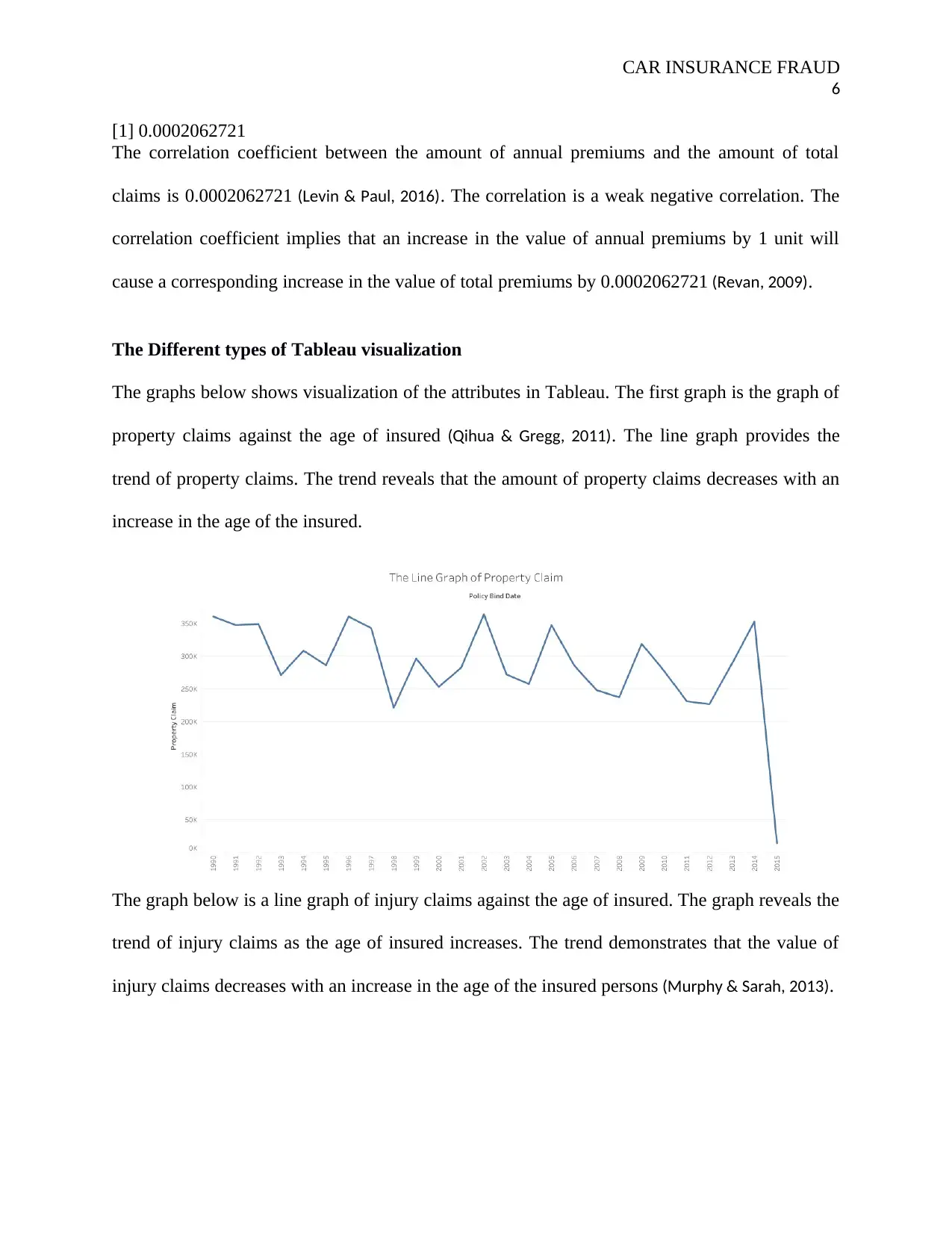
The graph below is a line graph of injury claims against the age of insured. The graph reveals the
trend of injury claims as the age of insured increases. The trend demonstrates that the value of
injury claims decreases with an increase in the age of the insured persons (Murphy & Sarah, 2013).
6
[1] 0.0002062721
The correlation coefficient between the amount of annual premiums and the amount of total
claims is 0.0002062721 (Levin & Paul, 2016). The correlation is a weak negative correlation. The
correlation coefficient implies that an increase in the value of annual premiums by 1 unit will
cause a corresponding increase in the value of total premiums by 0.0002062721 (Revan, 2009).
The Different types of Tableau visualization
The graphs below shows visualization of the attributes in Tableau. The first graph is the graph of
property claims against the age of insured (Qihua & Gregg, 2011). The line graph provides the
trend of property claims. The trend reveals that the amount of property claims decreases with an
increase in the age of the insured.
The graph below is a line graph of injury claims against the age of insured. The graph reveals the
trend of injury claims as the age of insured increases. The trend demonstrates that the value of
injury claims decreases with an increase in the age of the insured persons (Murphy & Sarah, 2013).
⊘ This is a preview!⊘
Do you want full access?
Subscribe today to unlock all pages.
Trusted by 1+ million students worldwide
CAR INSURANCE FRAUD
7
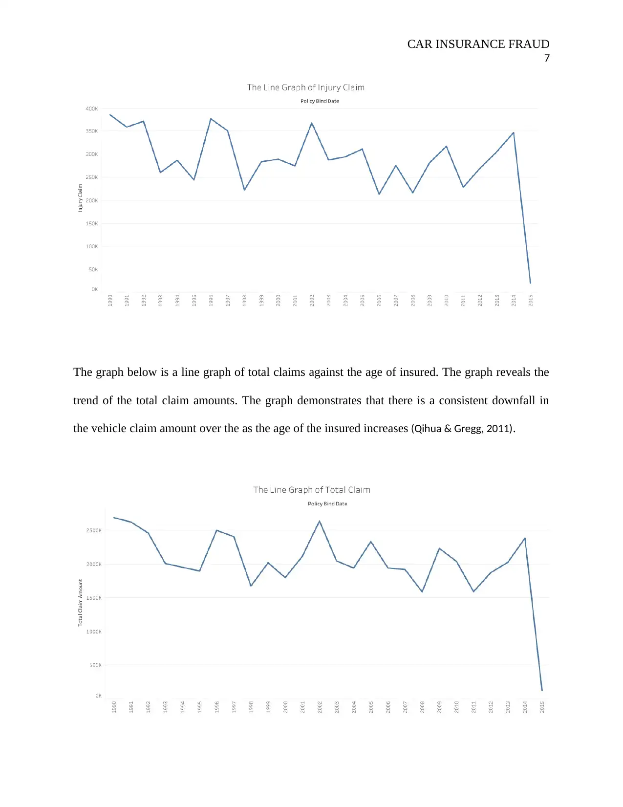
The graph below is a line graph of total claims against the age of insured. The graph reveals the
trend of the total claim amounts. The graph demonstrates that there is a consistent downfall in
the vehicle claim amount over the as the age of the insured increases (Qihua & Gregg, 2011).
7
The graph below is a line graph of total claims against the age of insured. The graph reveals the
trend of the total claim amounts. The graph demonstrates that there is a consistent downfall in
the vehicle claim amount over the as the age of the insured increases (Qihua & Gregg, 2011).
Paraphrase This Document
Need a fresh take? Get an instant paraphrase of this document with our AI Paraphraser
CAR INSURANCE FRAUD
8
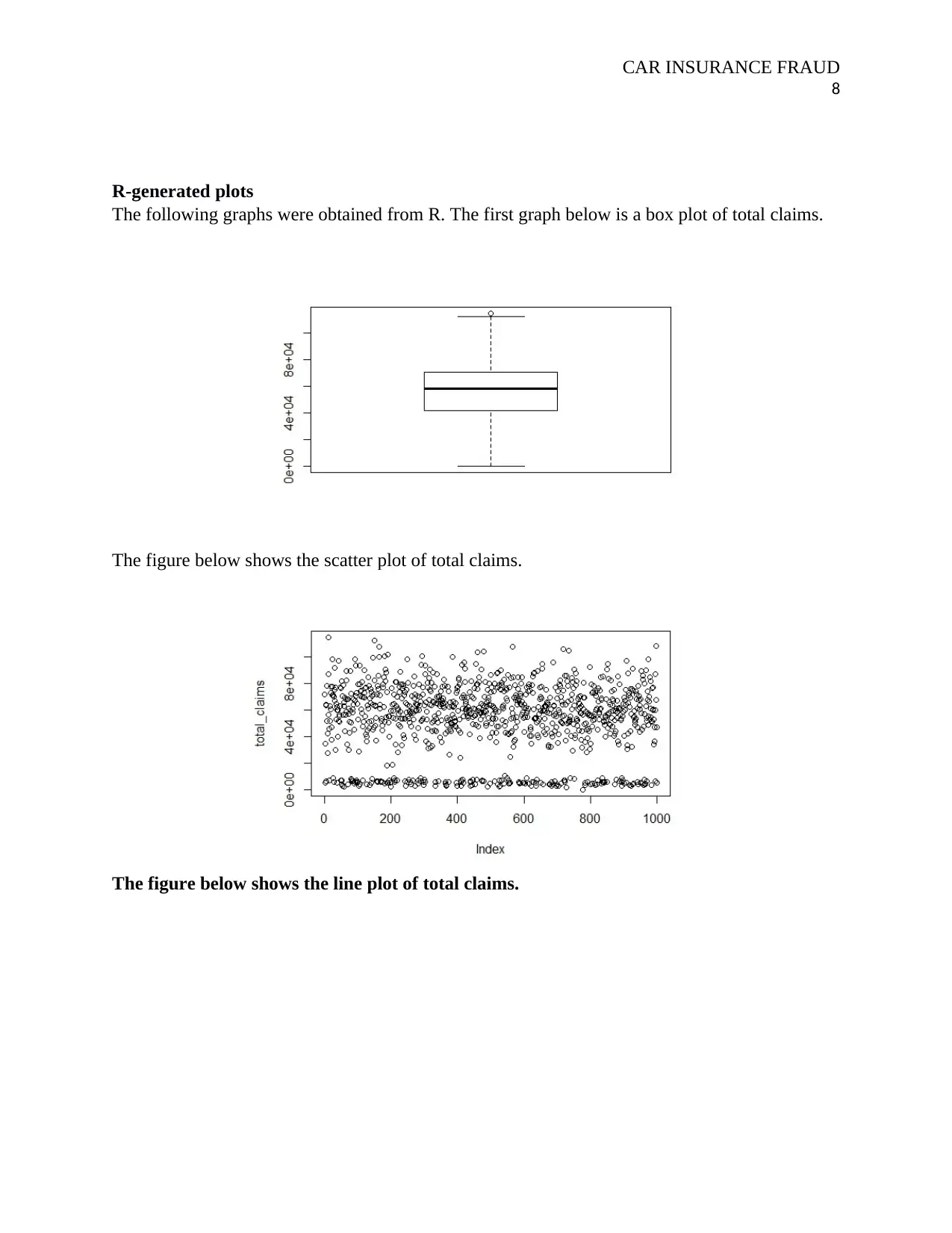
R-generated plots
The following graphs were obtained from R. The first graph below is a box plot of total claims.
The figure below shows the scatter plot of total claims.
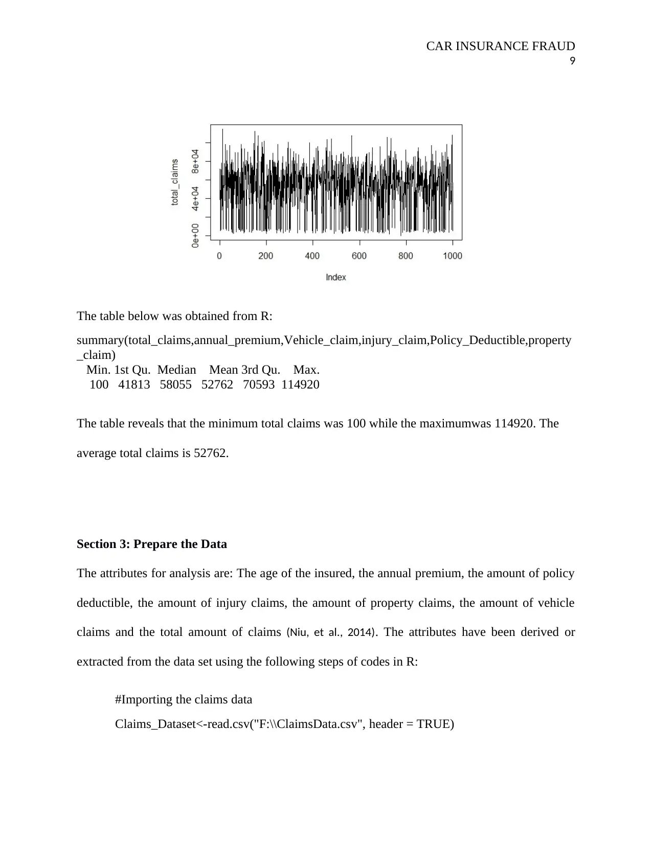
The figure below shows the line plot of total claims.
8
R-generated plots
The following graphs were obtained from R. The first graph below is a box plot of total claims.
The figure below shows the scatter plot of total claims.
The figure below shows the line plot of total claims.
CAR INSURANCE FRAUD
9
The table below was obtained from R:
summary(total_claims,annual_premium,Vehicle_claim,injury_claim,Policy_Deductible,property
_claim)
Min. 1st Qu. Median Mean 3rd Qu. Max.
100 41813 58055 52762 70593 114920
The table reveals that the minimum total claims was 100 while the maximumwas 114920. The
average total claims is 52762.
Section 3: Prepare the Data
The attributes for analysis are: The age of the insured, the annual premium, the amount of policy
deductible, the amount of injury claims, the amount of property claims, the amount of vehicle
claims and the total amount of claims (Niu, et al., 2014). The attributes have been derived or
extracted from the data set using the following steps of codes in R:
#Importing the claims data
Claims_Dataset<-read.csv("F:\\ClaimsData.csv", header = TRUE)
⊘ This is a preview!⊘
Do you want full access?
Subscribe today to unlock all pages.
Trusted by 1+ million students worldwide
CAR INSURANCE FRAUD
10
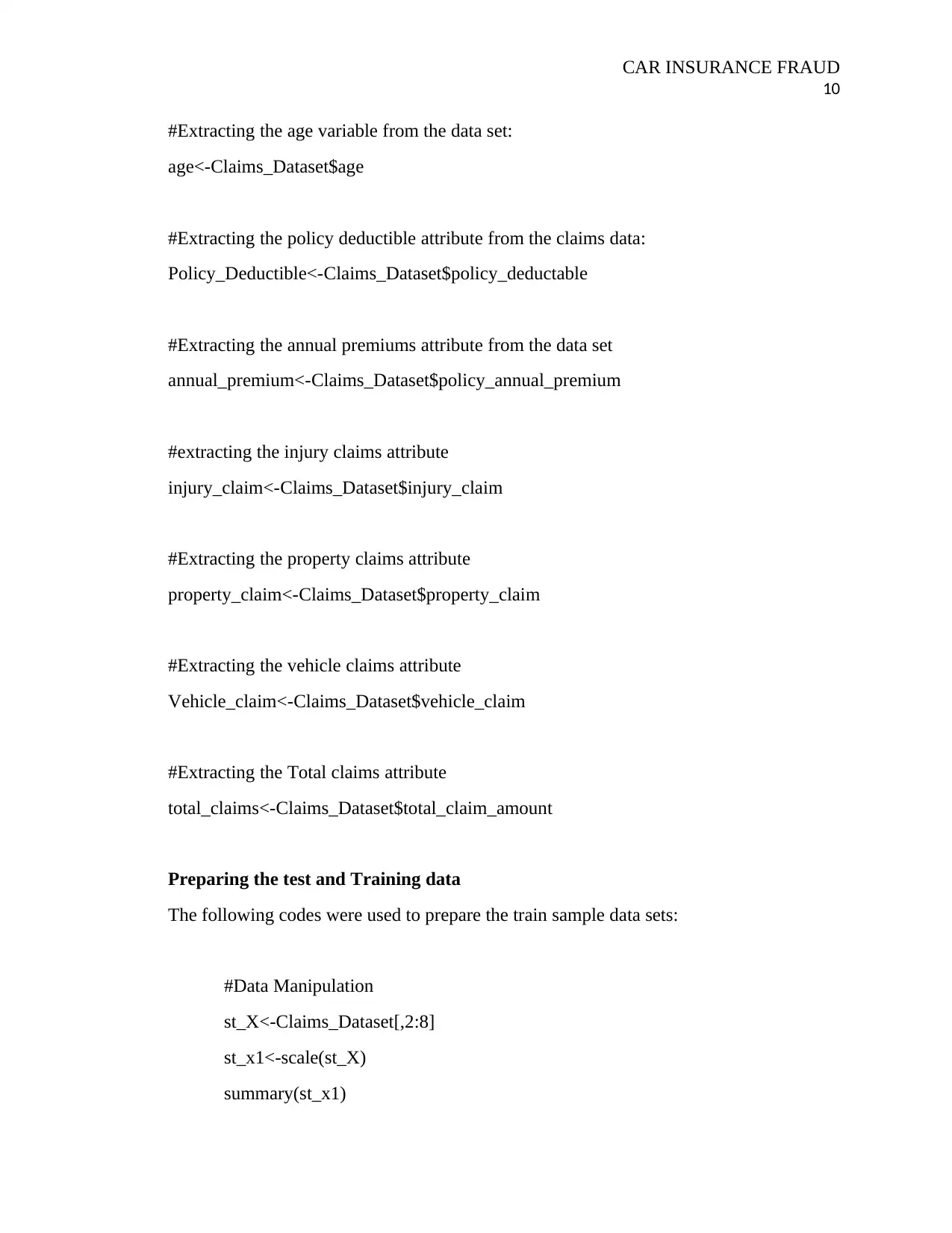
#Extracting the age variable from the data set:
age<-Claims_Dataset$age
#Extracting the policy deductible attribute from the claims data:
Policy_Deductible<-Claims_Dataset$policy_deductable
#Extracting the annual premiums attribute from the data set
annual_premium<-Claims_Dataset$policy_annual_premium
#extracting the injury claims attribute
injury_claim<-Claims_Dataset$injury_claim
#Extracting the property claims attribute
property_claim<-Claims_Dataset$property_claim
#Extracting the vehicle claims attribute
Vehicle_claim<-Claims_Dataset$vehicle_claim
#Extracting the Total claims attribute
total_claims<-Claims_Dataset$total_claim_amount
Preparing the test and Training data
The following codes were used to prepare the train sample data sets:
#Data Manipulation
st_X<-Claims_Dataset[,2:8]
st_x1<-scale(st_X)
summary(st_x1)
10
#Extracting the age variable from the data set:
age<-Claims_Dataset$age
#Extracting the policy deductible attribute from the claims data:
Policy_Deductible<-Claims_Dataset$policy_deductable
#Extracting the annual premiums attribute from the data set
annual_premium<-Claims_Dataset$policy_annual_premium
#extracting the injury claims attribute
injury_claim<-Claims_Dataset$injury_claim
#Extracting the property claims attribute
property_claim<-Claims_Dataset$property_claim
#Extracting the vehicle claims attribute
Vehicle_claim<-Claims_Dataset$vehicle_claim
#Extracting the Total claims attribute
total_claims<-Claims_Dataset$total_claim_amount
Preparing the test and Training data
The following codes were used to prepare the train sample data sets:
#Data Manipulation
st_X<-Claims_Dataset[,2:8]
st_x1<-scale(st_X)
summary(st_x1)
Paraphrase This Document
Need a fresh take? Get an instant paraphrase of this document with our AI Paraphraser
CAR INSURANCE FRAUD
11
library(class)
n<-nrow(Claims_Dataset)
#train datasets
train_data<-sample(n,0.7*n)
train_X<-st_x1[train_data]
train_Y<-Claims_Dataset[train_data,5]
#test datasets
test_X<-st_x1[-train_data]
test_Y<-Claims_Dataset[-train_data,5]
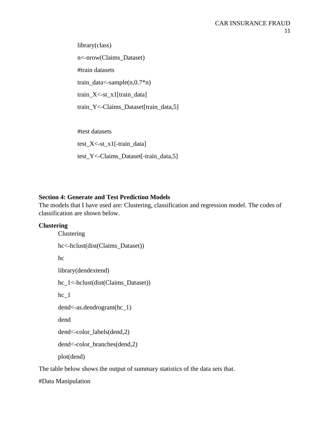
Section 4: Generate and Test Prediction Models
The models that I have used are: Clustering, classification and regression model. The codes of
classification are shown below.
Clustering
Clustering
hc<-hclust(dist(Claims_Dataset))
hc
library(dendextend)
hc_1<-hclust(dist(Claims_Dataset))
hc_1
dend<-as.dendrogram(hc_1)
dend
dend<-color_labels(dend,2)
dend<-color_branches(dend,2)
plot(dend)
The table below shows the output of summary statistics of the data sets that.
#Data Manipulation
11
library(class)
n<-nrow(Claims_Dataset)
#train datasets
train_data<-sample(n,0.7*n)
train_X<-st_x1[train_data]
train_Y<-Claims_Dataset[train_data,5]
#test datasets
test_X<-st_x1[-train_data]
test_Y<-Claims_Dataset[-train_data,5]
Section 4: Generate and Test Prediction Models
The models that I have used are: Clustering, classification and regression model. The codes of
classification are shown below.
Clustering
Clustering
hc<-hclust(dist(Claims_Dataset))
hc
library(dendextend)
hc_1<-hclust(dist(Claims_Dataset))
hc_1
dend<-as.dendrogram(hc_1)
dend
dend<-color_labels(dend,2)
dend<-color_branches(dend,2)
plot(dend)
The table below shows the output of summary statistics of the data sets that.
#Data Manipulation
CAR INSURANCE FRAUD
12
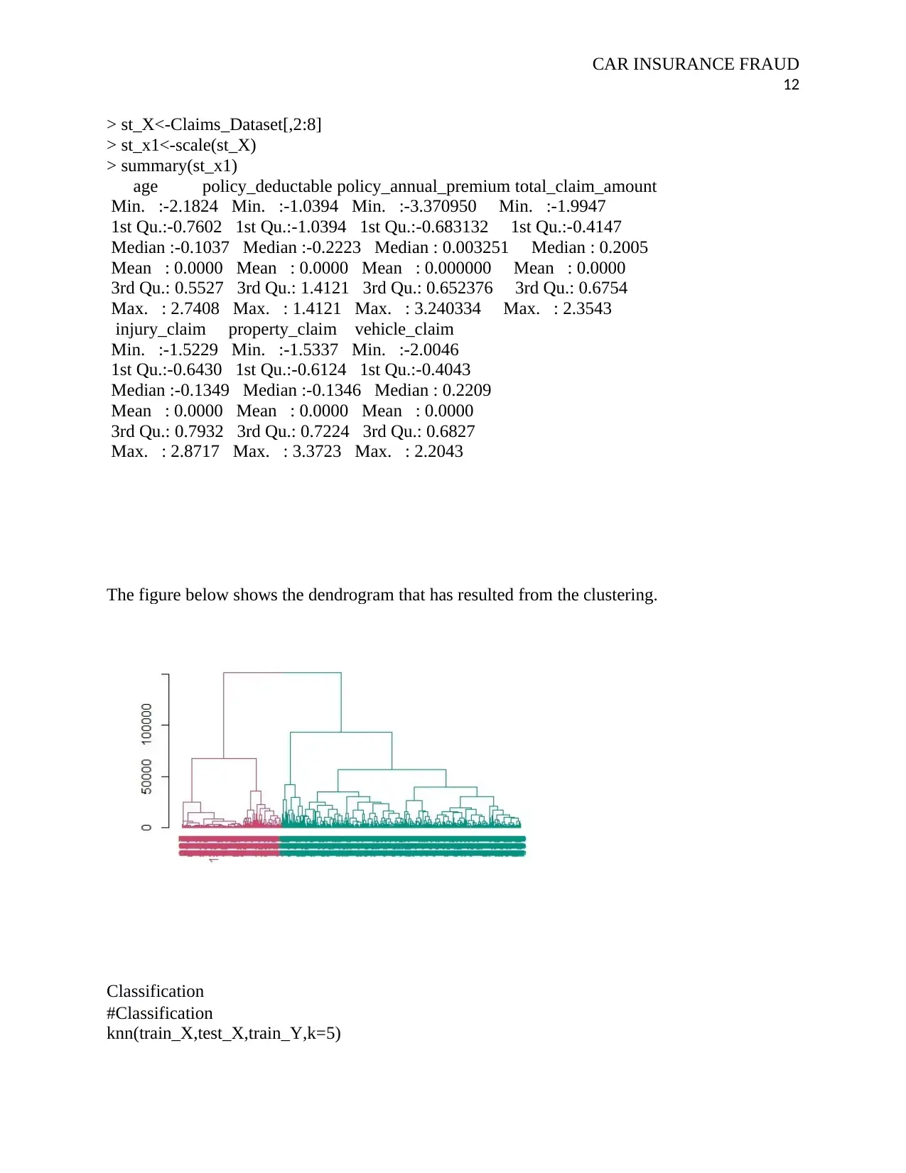
> st_X<-Claims_Dataset[,2:8]
> st_x1<-scale(st_X)
> summary(st_x1)
age policy_deductable policy_annual_premium total_claim_amount
Min. :-2.1824 Min. :-1.0394 Min. :-3.370950 Min. :-1.9947
1st Qu.:-0.7602 1st Qu.:-1.0394 1st Qu.:-0.683132 1st Qu.:-0.4147
Median :-0.1037 Median :-0.2223 Median : 0.003251 Median : 0.2005
Mean : 0.0000 Mean : 0.0000 Mean : 0.000000 Mean : 0.0000
3rd Qu.: 0.5527 3rd Qu.: 1.4121 3rd Qu.: 0.652376 3rd Qu.: 0.6754
Max. : 2.7408 Max. : 1.4121 Max. : 3.240334 Max. : 2.3543
injury_claim property_claim vehicle_claim
Min. :-1.5229 Min. :-1.5337 Min. :-2.0046
1st Qu.:-0.6430 1st Qu.:-0.6124 1st Qu.:-0.4043
Median :-0.1349 Median :-0.1346 Median : 0.2209
Mean : 0.0000 Mean : 0.0000 Mean : 0.0000
3rd Qu.: 0.7932 3rd Qu.: 0.7224 3rd Qu.: 0.6827
Max. : 2.8717 Max. : 3.3723 Max. : 2.2043
The figure below shows the dendrogram that has resulted from the clustering.
Classification
#Classification
knn(train_X,test_X,train_Y,k=5)
12
> st_X<-Claims_Dataset[,2:8]
> st_x1<-scale(st_X)
> summary(st_x1)
age policy_deductable policy_annual_premium total_claim_amount
Min. :-2.1824 Min. :-1.0394 Min. :-3.370950 Min. :-1.9947
1st Qu.:-0.7602 1st Qu.:-1.0394 1st Qu.:-0.683132 1st Qu.:-0.4147
Median :-0.1037 Median :-0.2223 Median : 0.003251 Median : 0.2005
Mean : 0.0000 Mean : 0.0000 Mean : 0.000000 Mean : 0.0000
3rd Qu.: 0.5527 3rd Qu.: 1.4121 3rd Qu.: 0.652376 3rd Qu.: 0.6754
Max. : 2.7408 Max. : 1.4121 Max. : 3.240334 Max. : 2.3543
injury_claim property_claim vehicle_claim
Min. :-1.5229 Min. :-1.5337 Min. :-2.0046
1st Qu.:-0.6430 1st Qu.:-0.6124 1st Qu.:-0.4043
Median :-0.1349 Median :-0.1346 Median : 0.2209
Mean : 0.0000 Mean : 0.0000 Mean : 0.0000
3rd Qu.: 0.7932 3rd Qu.: 0.7224 3rd Qu.: 0.6827
Max. : 2.8717 Max. : 3.3723 Max. : 2.2043
The figure below shows the dendrogram that has resulted from the clustering.
Classification
#Classification
knn(train_X,test_X,train_Y,k=5)
⊘ This is a preview!⊘
Do you want full access?
Subscribe today to unlock all pages.
Trusted by 1+ million students worldwide
1 out of 19


Your All-in-One AI-Powered Toolkit for Academic Success.
+13062052269
info@desklib.com
Available 24*7 on WhatsApp / Email
![[object Object]](/_next/static/media/star-bottom.7253800d.svg)
Unlock your academic potential
Copyright © 2020–2026 A2Z Services. All Rights Reserved. Developed and managed by ZUCOL.