Exploring Thermal Conductivity in Composite Materials
VerifiedAdded on 2020/04/21
|17
|3876
|417
AI Summary
The study centers around understanding the thermal properties of composite materials, especially those incorporating carbon nanotube structures. The focus is on how these composites can be optimized for better heat dissipation in practical applications such as automotive engines. Several methodologies and experimental designs are discussed, including steady state measurement devices and inverse problem solutions. The research highlights the significance of material selection—such as aluminum due to its high thermal conductivity—and examines various enhancements using carbon nanotubes. The broader implications consider how these findings can be applied to improve energy efficiency and performance in engineering applications.
Methodology on thermal conductivity measurement 1
METHODOLOGY ON THERMAL CONDUCTIVITY MESUREMENT
By Name
Course
Instructor
Institution
Location
Date
METHODOLOGY ON THERMAL CONDUCTIVITY MESUREMENT
By Name
Course
Instructor
Institution
Location
Date
Paraphrase This Document
Need a fresh take? Get an instant paraphrase of this document with our AI Paraphraser
Methodology on thermal conductivity measurement 2
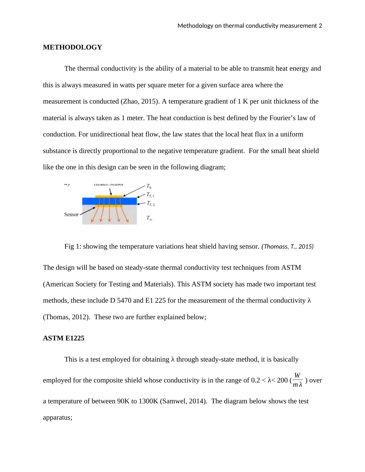
METHODOLOGY
The thermal conductivity is the ability of a material to be able to transmit heat energy and
this is always measured in watts per square meter for a given surface area where the
measurement is conducted (Zhao, 2015). A temperature gradient of 1 K per unit thickness of the
material is always taken as 1 meter. The heat conduction is best defined by the Fourier’s law of
conduction. For unidirectional heat flow, the law states that the local heat flux in a uniform
substance is directly proportional to the negative temperature gradient. For the small heat shield
like the one in this design can be seen in the following diagram;
Fig 1: showing the temperature variations heat shield having sensor. (Thomass, T., 2015)
The design will be based on steady-state thermal conductivity test techniques from ASTM
(American Society for Testing and Materials). This ASTM society has made two important test
methods, these include D 5470 and E1 225 for the measurement of the thermal conductivity λ
(Thomas, 2012). These two are further explained below;
ASTM E1225
This is a test employed for obtaining λ through steady-state method, it is basically
employed for the composite shield whose conductivity is in the range of 0.2 < λ< 200 ( W
m λ ) over
a temperature of between 90K to 1300K (Samwel, 2014). The diagram below shows the test
apparatus;
Methodology on thermal conductivity measurement 3
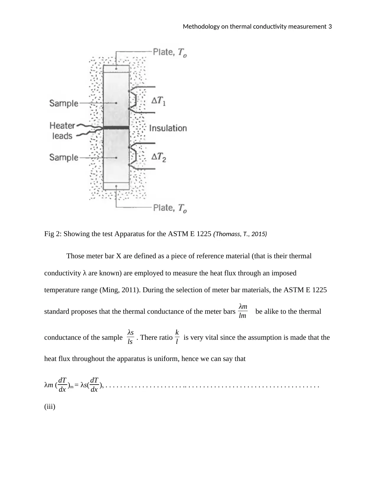
Fig 2: Showing the test Apparatus for the ASTM E 1225 (Thomass, T., 2015)
Those meter bar X are defined as a piece of reference material (that is their thermal
conductivity λ are known) are employed to measure the heat flux through an imposed
temperature range (Ming, 2011). During the selection of meter bar materials, the ASTM E 1225
standard proposes that the thermal conductance of the meter bars λm
lm be alike to the thermal
conductance of the sample λs
ls . There ratio k
l is very vital since the assumption is made that the
heat flux throughout the apparatus is uniform, hence we can say that
λm ( dT
dx )m = λs( dT
dx )s . . . . . . . . . . . . . . . . . . . . . .. . . . . . . . . . . . . . . . . . . . . . . . . . . . . . . . . . . . .
(iii)
⊘ This is a preview!⊘
Do you want full access?
Subscribe today to unlock all pages.
Trusted by 1+ million students worldwide
Methodology on thermal conductivity measurement 4
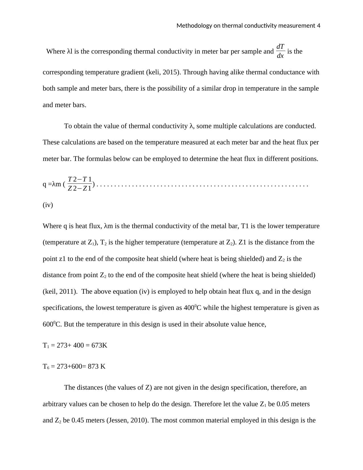
Where λl is the corresponding thermal conductivity in meter bar per sample and dT
dx is the
corresponding temperature gradient (keli, 2015). Through having alike thermal conductance with
both sample and meter bars, there is the possibility of a similar drop in temperature in the sample
and meter bars.
To obtain the value of thermal conductivity λ, some multiple calculations are conducted.
These calculations are based on the temperature measured at each meter bar and the heat flux per
meter bar. The formulas below can be employed to determine the heat flux in different positions.
q =λm ( T 2−T 1
Z 2−Z 1 ) . . . . . . . . . . . . . . . . . . . . . . . . . . . . . . . . . . . . . . . . . . . . . . . . . . . . . . . . . . . .
(iv)
Where q is heat flux, λm is the thermal conductivity of the metal bar, T1 is the lower temperature
(temperature at Z1), T2 is the higher temperature (temperature at Z2). Z1 is the distance from the
point z1 to the end of the composite heat shield (where heat is being shielded) and Z2 is the
distance from point Z2 to the end of the composite heat shield (where the heat is being shielded)
(keil, 2011). The above equation (iv) is employed to help obtain heat flux q, and in the design
specifications, the lowest temperature is given as 4000C while the highest temperature is given as
6000C. But the temperature in this design is used in their absolute value hence,
T1 = 273+ 400 = 673K
T6 = 273+600= 873 K
The distances (the values of Z) are not given in the design specification, therefore, an
arbitrary values can be chosen to help do the design. Therefore let the value Z1 be 0.05 meters
and Z2 be 0.45 meters (Jessen, 2010). The most common material employed in this design is the
Paraphrase This Document
Need a fresh take? Get an instant paraphrase of this document with our AI Paraphraser
Methodology on thermal conductivity measurement 5
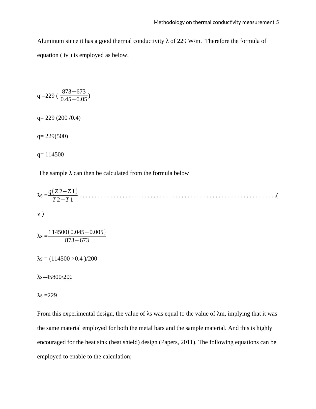
Aluminum since it has a good thermal conductivity λ of 229 W/m. Therefore the formula of
equation ( iv ) is employed as below.
q =229 ( 873−673
0.45−0.05 )
q= 229 (200 /0.4)
q= 229(500)
q= 114500
The sample λ can then be calculated from the formula below
λs = q( Z 2−Z 1)
T 2−T 1 . . . . . . . . . . . . . . . . . . . . . . . . . . . . . . . . . . . . . . . . . . . . . . . . . . . . . . . . . . . . . . . .(
v )
λs = 114500(0.045−0.005)
873−673
λs = (114500 ×0.4 )/200
λs=45800/200
λs =229
From this experimental design, the value of λs was equal to the value of λm, implying that it was
the same material employed for both the metal bars and the sample material. And this is highly
encouraged for the heat sink (heat shield) design (Papers, 2011). The following equations can be
employed to enable to the calculation;
Methodology on thermal conductivity measurement 6
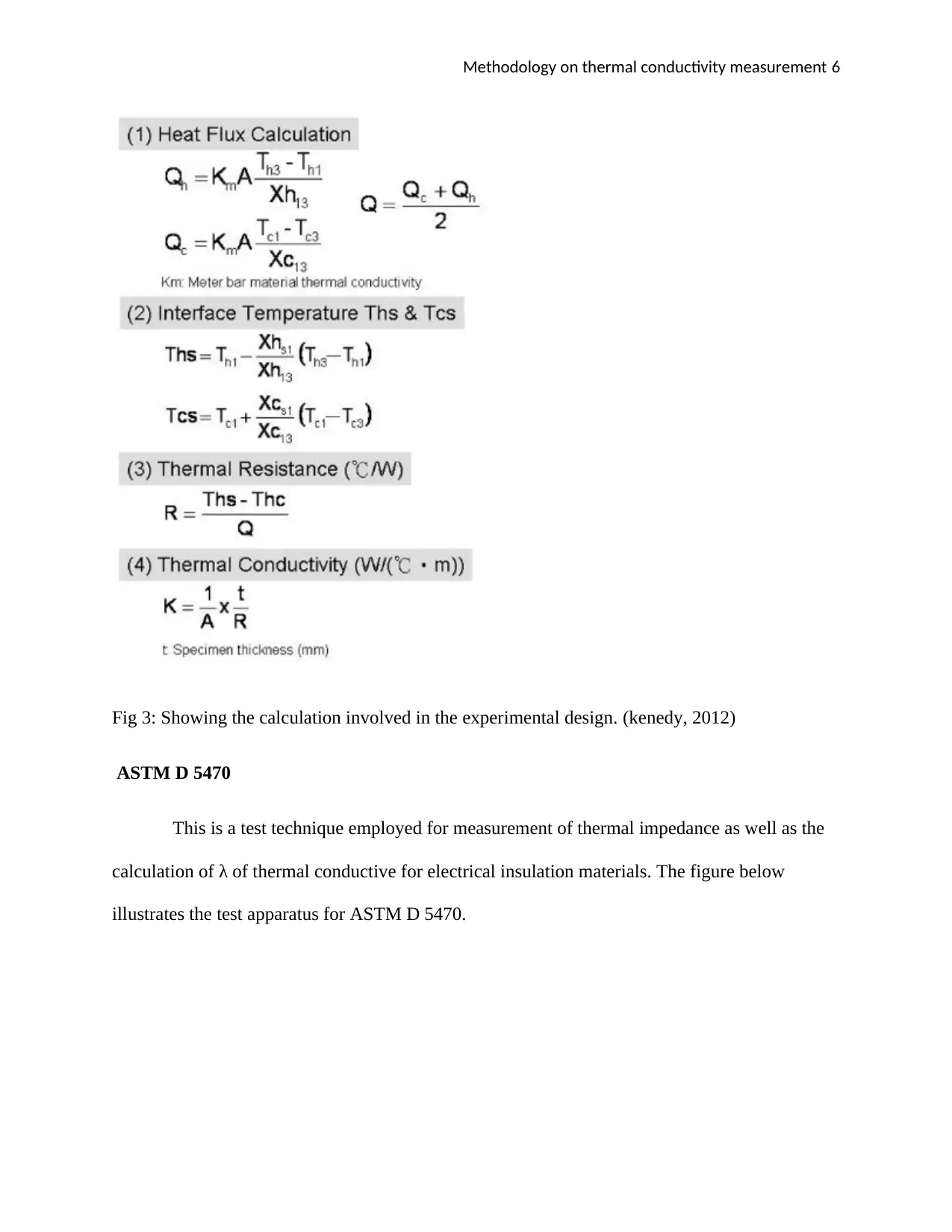
Fig 3: Showing the calculation involved in the experimental design. (kenedy, 2012)
ASTM D 5470
This is a test technique employed for measurement of thermal impedance as well as the
calculation of λ of thermal conductive for electrical insulation materials. The figure below
illustrates the test apparatus for ASTM D 5470.
⊘ This is a preview!⊘
Do you want full access?
Subscribe today to unlock all pages.
Trusted by 1+ million students worldwide
Methodology on thermal conductivity measurement 7
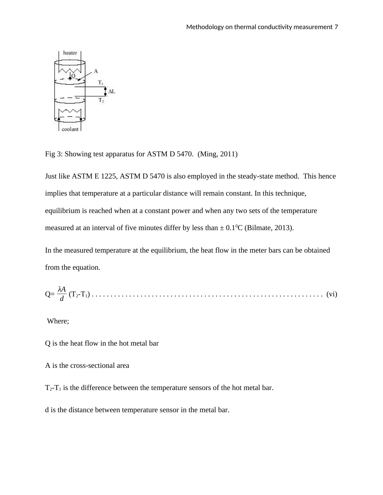
Fig 3: Showing test apparatus for ASTM D 5470. (Ming, 2011)
Just like ASTM E 1225, ASTM D 5470 is also employed in the steady-state method. This hence
implies that temperature at a particular distance will remain constant. In this technique,
equilibrium is reached when at a constant power and when any two sets of the temperature
measured at an interval of five minutes differ by less than ± 0.10C (Bilmate, 2013).
In the measured temperature at the equilibrium, the heat flow in the meter bars can be obtained
from the equation.
Q= λA
d (T2-T1) . . . . . . . . . . . . . . . . . . . . . . . . . . . . . . . . . . . . . . . . . . . . . . . . . . . . . . . . . . . . . . (vi)
Where;
Q is the heat flow in the hot metal bar
A is the cross-sectional area
T2-T1 is the difference between the temperature sensors of the hot metal bar.
d is the distance between temperature sensor in the metal bar.
Paraphrase This Document
Need a fresh take? Get an instant paraphrase of this document with our AI Paraphraser
Methodology on thermal conductivity measurement 8
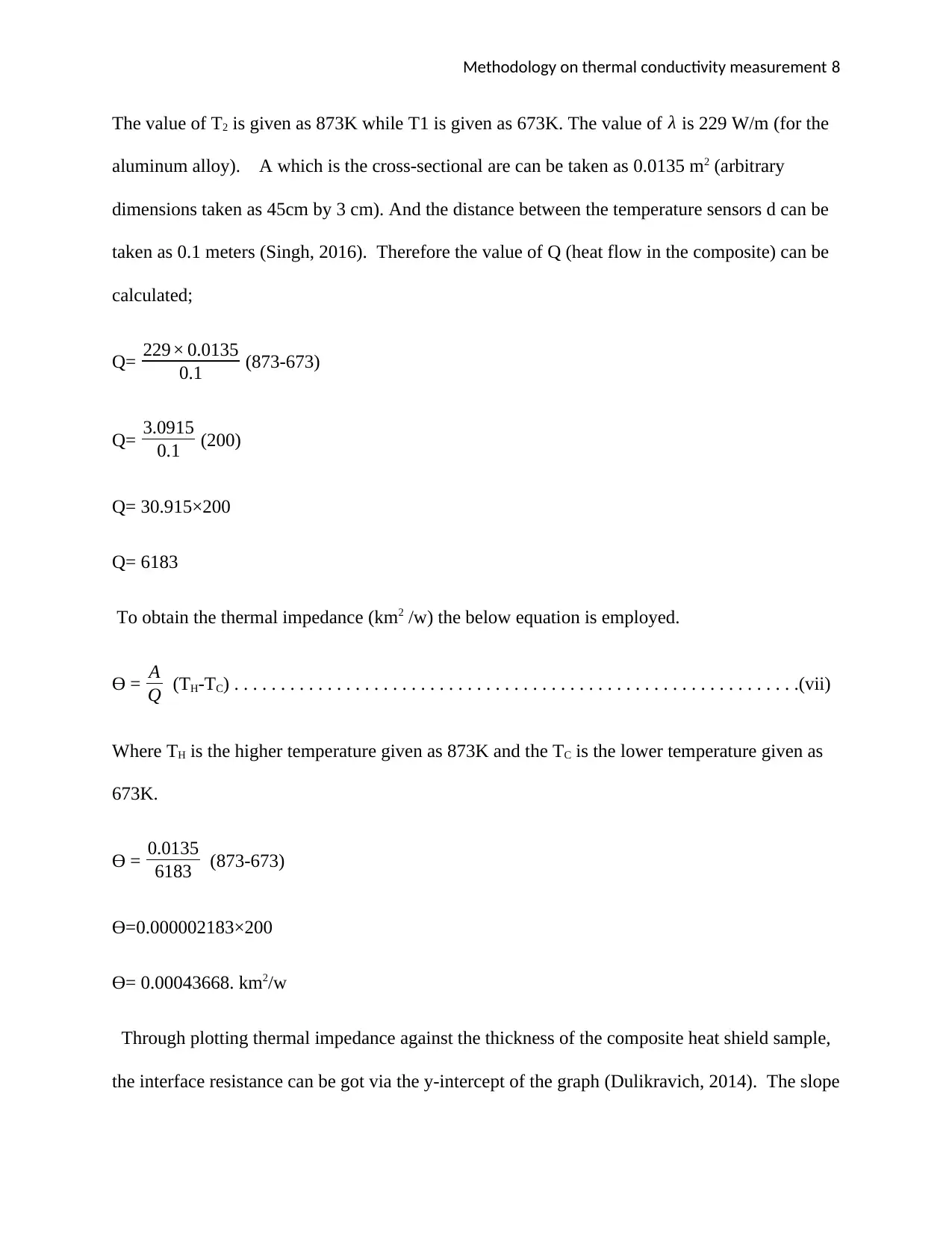
The value of T2 is given as 873K while T1 is given as 673K. The value of λ is 229 W/m (for the
aluminum alloy). A which is the cross-sectional are can be taken as 0.0135 m2 (arbitrary
dimensions taken as 45cm by 3 cm). And the distance between the temperature sensors d can be
taken as 0.1 meters (Singh, 2016). Therefore the value of Q (heat flow in the composite) can be
calculated;
Q= 229× 0.0135
0.1 (873-673)
Q= 3.0915
0.1 (200)
Q= 30.915×200
Q= 6183
To obtain the thermal impedance (km2 /w) the below equation is employed.
ϴ = A
Q (TH-TC) . . . . . . . . . . . . . . . . . . . . . . . . . . . . . . . . . . . . . . . . . . . . . . . . . . . . . . . . . . . . .(vii)
Where TH is the higher temperature given as 873K and the TC is the lower temperature given as
673K.
ϴ = 0.0135
6183 (873-673)
ϴ=0.000002183×200
ϴ= 0.00043668. km2/w
Through plotting thermal impedance against the thickness of the composite heat shield sample,
the interface resistance can be got via the y-intercept of the graph (Dulikravich, 2014). The slope
Methodology on thermal conductivity measurement 9
of the graph will give the reciprocal of the thermal conductivity λ of the composite heat sink heat
shield).
To affirm the precision of these ASTM test techniques, the methodology of a round
robin is implemented with six different laboratories and five materials. From several
experimental designs data obtained, it can be concluded that the value of thermal conductivity λ
for the similar materials measured in different laboratories, the value of λ is 18% from one
another. Therefore, this will confirm the overall accuracy thermal conductivity measurement
using the ASTM techniques and standards (Dilling, 2013).
INITIAL TEST APPARATUS
The initial experimental design was conducted using the two ASTM shown above where both
methods used Fourier’s Law. The meter bars are of the standard material (known material), thus
the heat flux (Q/A) moving via the meter bar can easily be estimated and the value of λ can be
obtained from the below equation;
λ= - Q
A
dx
dT . . . . . . . . . . . . . . . . . . . . . . . . . . . . . . . . . . . . . . . . . . . . . . . . . . . . . . . . . . . . . . . . (viii)
The diagram below shows the schematic for this experimental design;
⊘ This is a preview!⊘
Do you want full access?
Subscribe today to unlock all pages.
Trusted by 1+ million students worldwide
Methodology on thermal conductivity measurement 10
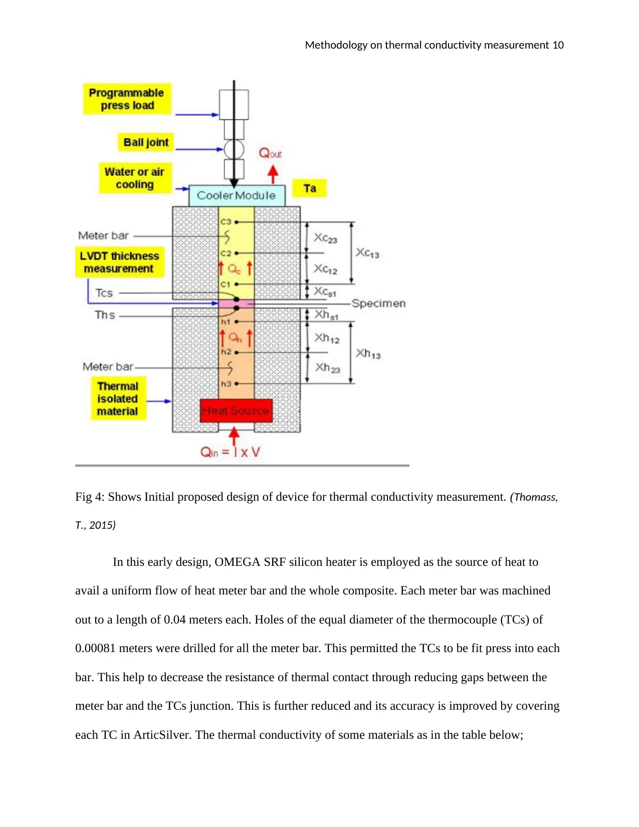
Fig 4: Shows Initial proposed design of device for thermal conductivity measurement. (Thomass,
T., 2015)
In this early design, OMEGA SRF silicon heater is employed as the source of heat to
avail a uniform flow of heat meter bar and the whole composite. Each meter bar was machined
out to a length of 0.04 meters each. Holes of the equal diameter of the thermocouple (TCs) of
0.00081 meters were drilled for all the meter bar. This permitted the TCs to be fit press into each
bar. This help to decrease the resistance of thermal contact through reducing gaps between the
meter bar and the TCs junction. This is further reduced and its accuracy is improved by covering
each TC in ArticSilver. The thermal conductivity of some materials as in the table below;
Paraphrase This Document
Need a fresh take? Get an instant paraphrase of this document with our AI Paraphraser
Methodology on thermal conductivity measurement 11
No Wire material λ ( W/mK)
1 Aluminum alloy 229
2 Iron 73
3 Alumel 48
4 Constantan 23
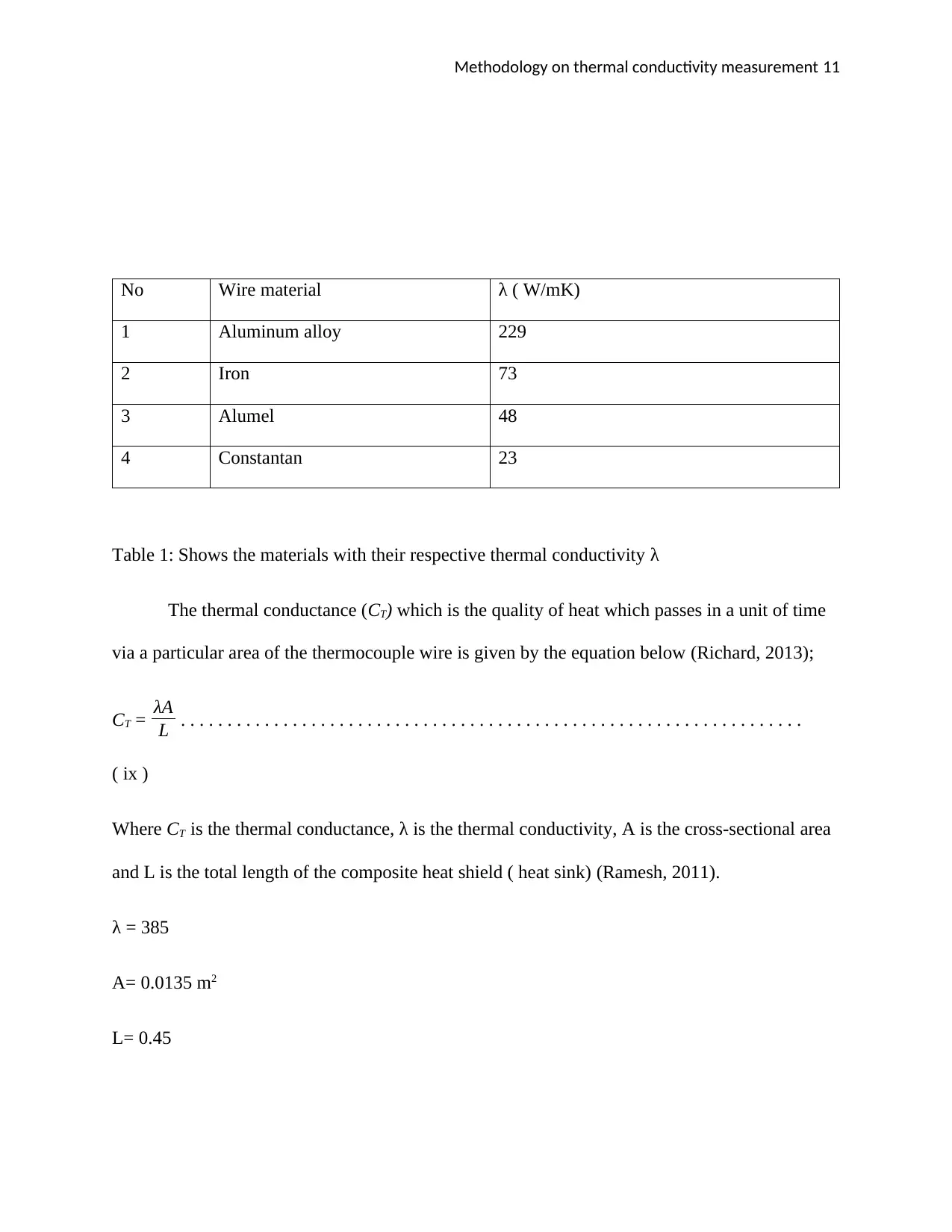
Table 1: Shows the materials with their respective thermal conductivity λ
The thermal conductance (CT) which is the quality of heat which passes in a unit of time
via a particular area of the thermocouple wire is given by the equation below (Richard, 2013);
CT = λA
L . . . . . . . . . . . . . . . . . . . . . . . . . . . . . . . . . . . . . . . . . . . . . . . . . . . . . . . . . . . . . . . . . . .
( ix )
Where CT is the thermal conductance, λ is the thermal conductivity, A is the cross-sectional area
and L is the total length of the composite heat shield ( heat sink) (Ramesh, 2011).
λ = 385
A= 0.0135 m2
L= 0.45
No Wire material λ ( W/mK)
1 Aluminum alloy 229
2 Iron 73
3 Alumel 48
4 Constantan 23
Table 1: Shows the materials with their respective thermal conductivity λ
The thermal conductance (CT) which is the quality of heat which passes in a unit of time
via a particular area of the thermocouple wire is given by the equation below (Richard, 2013);
CT = λA
L . . . . . . . . . . . . . . . . . . . . . . . . . . . . . . . . . . . . . . . . . . . . . . . . . . . . . . . . . . . . . . . . . . .
( ix )
Where CT is the thermal conductance, λ is the thermal conductivity, A is the cross-sectional area
and L is the total length of the composite heat shield ( heat sink) (Ramesh, 2011).
λ = 385
A= 0.0135 m2
L= 0.45

Methodology on thermal conductivity measurement 12
CT = 385× 0.0135
0.45
CT = 5.1975
0.45
CT = 11.55
FINAL EXPERIMENTAL DESIGN
After the initial experimental design, the whole design is made more realistic in the final
experimental design. The final design diagram is shown in the figure;
Fig 5: Shows the final design of a device for thermal conductivity measurement. (Thomass, T.,
2015)
⊘ This is a preview!⊘
Do you want full access?
Subscribe today to unlock all pages.
Trusted by 1+ million students worldwide
1 out of 17
Your All-in-One AI-Powered Toolkit for Academic Success.
+13062052269
info@desklib.com
Available 24*7 on WhatsApp / Email
![[object Object]](/_next/static/media/star-bottom.7253800d.svg)
Unlock your academic potential
Copyright © 2020–2026 A2Z Services. All Rights Reserved. Developed and managed by ZUCOL.