ECON 2009H Managerial Economics: Winter 2020 Final Exam Solution
VerifiedAdded on 2022/07/28
|18
|3362
|22
Homework Assignment
AI Summary
This document presents a comprehensive solution to the Managerial Economics ECON 2009H final take-home exam from Carleton University, Winter 2020. The exam covers a range of topics including consumer behavior, market equilibrium, and firm strategies. The solution begins with an analysis of consumer choice under different price and income scenarios, illustrating the impact on budget lines and utility maximization. It then delves into market structures, specifically perfect competition and duopoly, calculating industry output, firm profits, and the effects of market shifts. Furthermore, the solution addresses decision-making under uncertainty, analyzing an investor's willingness to pay for information and the pricing strategies for a newsletter. Finally, it examines the Cournot oligopoly model, determining equilibrium quantities, market prices, and profits for firms, both in competitive and collusive scenarios.

INSTRUCTIONS
Make sure to write your name and ID in the first page and every page
thereafter.
The question booklet consists of 15 pages. Make sure you have all of
them.
Answer the questions in the spaces provided after each question. If you
run out ofroom for an answer, continue on a
blank page.
The mark of each question is printed next to it.
Make sure you read and sign the Declaration Of Academic Integrity
shown below.
Declaration of Academic Integrity
ectations and prohibitions set by the course instructor. In particular, in writing this exam, I
others. I understand that any breach of these terms, or breach from the terms of the Acade
Signature: . . . . . . . . . . . . . . . . . . . . . . . . . . . . . . . . . . . . . . . . . . . . . . . . . . . . . . . . . . . . . .
CARLETON UNIVERSITY
Final Take-Home Exam Winter 2020
Course Title: Managerial Economics Course Number: ECON 2009 H Course
Instructor(s): Mumtaz Ahmad
Name: University ID:
Question: Total
Points:
Score:
1
Paraphrase This Document
Need a fresh take? Get an instant paraphrase of this document with our AI Paraphraser

Nam
e:
Managerial Economics
2009 H
Page 2 of
15
1. Suppose that the following graph represents the optimal consumption bundle of a typical consumer, with an
income of 80, facing prices PX = 1 and PY = 1 and with utility U=XY. Figure 1
(a) 4Now, let income remain fixed let prices rise so that PX = 2, PY = 4. Illustrate the new budget line and draw a
sample indifference curve to show the new equilibrium bundle.
Y
80 Figure 2
M=budget line
40 K1
` 30 K2 U1
U2
40 50 80 X
The consumer is subjected to two commodities, that is X and Y. An increase in the price of commodity X has no
effect on the quantity bought and consumed of commodity Y but would rather reduce the quantity consumed of
commodity X. since the price of Y has increased more than the price of X, it causes the budget constraint to curve
inwards as though it was pegged on a hinge (Quirmbach, Cornelsen, Jebb, Marteau, & Smith, 2018). The point of
intersection between the utility curve and the budget line shows the originally preferred bundle that yields optimal
utility to the consumer.

Nam
e:
Managerial Economics
2009 H
Page 3 of
15
(b) Let income be indexed to the cost of living so that budget line shifts out just enough that the old bundle (at the
original prices, above) is just affordable. In other words, let income increase to 240. Is the old bundle still the optimal
choice at the new income level and new prices? Has utility increased above that of the original consumption bundle?
Explain using a diagram.
240
I2
B
80 K
A C
40 I3
I1
40 80 240
The original bundle would not be the optimal choice as any decision to consume at B, C or K would
yield more utility as more of the commodities would be purchased by the consumer depending on his
personal preference.
(c) Suppose that prices are now PX = 2, PY = 2, and income has increased to 160 (so that both income and prices
have exactly doubled over the original levels). Is the old bundle optimal now? Has utility increased above that of the
original consumption bundle?
When the income of the consumer increases to 160 units, it would be expected that the budget line shifts rightwards,
from say Q1 to Q2 implying that more goods can be consumed as real income increases. However, when the prices
also double, the consumer would not be able to buy more of the items and therefore the budget line shifts backwards
to its original position. In simple words, there would be no change in the equilibrium position for the consumer.
⊘ This is a preview!⊘
Do you want full access?
Subscribe today to unlock all pages.
Trusted by 1+ million students worldwide

−
Managerial Economics
2009 H
Nam
e:
Page 4 of
15
2. Let total cost for each firm in perfectly competitive industry be TC(q) = 100 + q2 for positive q
and TC(q) = 0 for q = 0, and demand be Q D = 10000 − 100P . Answer the following questions.
(a) What will be industry output in long-run equilibrium?
Profit maximization occurs at the point where MC=MR subject to a linier demand curve where the MR has the same
vertical intercept as the AR and two time the slope.
We begin by expressing q in terms of p as follows:
From Q D = 10000 − 100P, when rearranged, we obtain 100p = 10,000- Q
P= 100- 0.01Q. From the explanation above we set MR=100-0.02Q
Since MC= dC/dQ, implying that MC= 2q, we set MC=MR
Hence, 100-0.02q =2q.
10,000-2q=200q
10,000=202q
Q= 49.501
(b) Suppose that demand is QD = 5000 50P . What is the industry output in long-run
equilibrium? How many firms will be there in the industry?
Express the equation in terms of p.
From qd= 5000 – 50p
50p= 5000- qd
P = 100-0.02q
Giving the MR = 100-0.04q
And that MC=2Q
From theory, MC=MR
100-0.04q = 2q
100= 2.04q
Q= 49.02
Number of firms
From 50p= 5000- qd
50p = 5000-q
P=100-0.02*49.02
P= 0.9804
Qd = 5000-50*0.9804
Since each firm maximizes output at Q= 49.02
The optimal number of firms in the market would be
4902/49.02
= 101 firms
Paraphrase This Document
Need a fresh take? Get an instant paraphrase of this document with our AI Paraphraser

−
Managerial Economics
2009 H
Nam
e:
Page 5 of
15
(c) Suppose that demand now shifts to be QD = 6000 - 50P but that it is not possible to manufacture more
(industry) output than the long-run equilibrium output in part (b). What is the new equilibrium price of output? How
much profit does manufacturer if each sets its output optimally given the new price and constraints in this setup?
P is given by the expression p=120 -0.02Q
P= 120-0.02*49.02
P= 120-0.9804
P= 119.02
Q= 600-0.02*119.02
Q= 600-2.3804
Q= 5970.16
The new profit
Profit =TR - TC
Remember that MR = MC
From MR=p*
MR= 120-0.04q
TR= 120- 0.02q2
Similarly MC= 2Q
TC= Q2
PROFIT = 120-0.04Q-Q2
PROFIT= 12000-4Q-100Q2
PROFIT= 12000-4(597.16)-100(597.16)
PROFIT = 9,000

Managerial Economics
2009 H
Nam
e:
Page 6 of
15
(d) In the long-run, how many new firms will enter in this industry when demand shifts as in part (c)?
Total output = 6000-50*1/3*120= 3872.58
Each firm produces 49.02
Number of firms is computed by
3872.58/49.02
=79 firms
2009 H
Nam
e:
Page 6 of
15
(d) In the long-run, how many new firms will enter in this industry when demand shifts as in part (c)?
Total output = 6000-50*1/3*120= 3872.58
Each firm produces 49.02
Number of firms is computed by
3872.58/49.02
=79 firms
⊘ This is a preview!⊘
Do you want full access?
Subscribe today to unlock all pages.
Trusted by 1+ million students worldwide

Managerial Economics
2009 H
Nam
e:
Page 7 of
15
3. An investor with a total wealth of $100 is faced with the following opportunities. First, he may invest $100 now
and receive $144 if there are good times, but receive $64 if there are bad times. The investor estimates that good
times happen with 50% probability. He can also buy an investor newsletter whether good times or bad times with
occur.
(a) Draw the decision tree that illustrates the options available to the investor and the payoffs to the different
options. Define P as the price of the newsletter.
0.5 0.5
(b) If the investor is risk-neutral with U (M ) = M , where M is income, how much would he be willing to pay for
the subscription to the newsletter?
A Risk-Neutral person whose certain equivalent of any gamble is just equivalent to its speculated monetary value
(EMV). A decision-maker’s certainty equivalent is the lowest monetary value that can be drawn from a transaction
instead of a gamble. He would be willing to pay
We establish the certainty equivalent (CE) – this is the lowest amount of money that the investor would be willing to
receive as return after investment.
From the report, we have
0.5*0.5*100= 25 during good experience and
0.5*0.5*64= 16 during the bad period
Since the expected equivalence of the investor is equal to the lowest expected return from the venture, the investor
would be willing to pay 16 units for newsletter subscription
InvestDon’t
Bad times (returns God times (returns
Buy
investment 0.50.5
Paraphrase This Document
Need a fresh take? Get an instant paraphrase of this document with our AI Paraphraser

Managerial Economics
2009 H
Nam
e:
Page 8 of
15
(c) If the investor is risk-averse with utility U (M ) = M 0.5, where M is income, how much would this investor be
willing to pay for the subscription to the newsletter?
Risk-averse situations are cases where an individual has the mind-set of focusing more on the fear of losing money
rather than the merits associated with more returns on investment. In other words, a person is risk-averse if his or her
action yields lesser returns compared to the gamble’s projected monetary rewards. When the gamble’s expected
monetary value is computed less the investor’s certainty equivalent, the result is the decision-making risk premium.
We compute RP= EMV – CE.
This can be computed as
The upper limit =144 with 0.5 probability
Lower limit = 64 with 0.5 probability
The risk premium is given by (144*1/2) – (64)
RP= 72-64
RP = 8
In our case,
We compute the expected utility
E(U) = PU(M)0.5
E(U) = PU(100)
E(U) = 8(100)0.5
E(U) = 80
Since expected utility is more than the returns during bad times but less than the returns in good time, the investor
would be willing to pay 8 units for newsletter subscription.

Managerial Economics
2009 H
Nam
e:
Page 9 of
15
(d) Suppose that the owner of the newsletter estimates that there are 75 risk-averse investors like those of part (c)
and 25 investors like those of part(b). If it costs zero to produce the newsletter, how should the newsletter be priced
assuming (i) that the owner wishes to maximize the profits of the newsletter and (ii) that this is the only newsletter
available to investors.
Risk neutral investors = 0.75
Risk-averse investors = 0.25
The newsletter owner should adopt a mixed pricing strategy as follows
Market price = 0.75* 16+ 0.25*8 = 14
The newsletter should be priced at 14 since the value is less than the value of the certainty equivalent in the larger market
segment.
⊘ This is a preview!⊘
Do you want full access?
Subscribe today to unlock all pages.
Trusted by 1+ million students worldwide

Managerial Economics
2009 H
Nam
e:
Page 10 of
15
4. Two firms, A and B, compete as duopolists in an industry. The firms produce a homogeneous good. Each firm
has a cost function given by:
C(q) = 30q + 1.5q2
The (inverse) market demand for the product can be written as:
P = 300 − 3Q
, where Q = q1 + q2, total output.
(a) If each firm acts to maximize its profits, taking its rival’s output as given (i.e., the firms behave as Cournot
oligopolists), what will be the equilibrium quantities selected by each firm? What is total output, and what is the
market price? What are the profits for each firm?
Profit maximization for an individual firm is given where:
For firm A: MRA = MCA
MCA is computed from
MCA = d(TCA )/ dQA
While MR is given by MR=P
TRA is computed from the expression
TRA = P*QL
TCA = 30QA+1.5QA2
PA= 300 − 3QA and
QA= 30QA + 1.5QA2
QA is computed based on the fact that firm B would sell as much of the product as it wishes given the market price (p). Firm B is
faced with the demand function expressed as MRB=P
To maximize profit, firm B will operate at the point where MR=MC
300-3q=30+3q
6q=270
Q= 45
P= 300-30*45
P= 165
Total output
Q=q1+q2
Q1= 100-1/3p
Q1 =100-55
Q1= 45
Q2= 100-1/3p
Q2 = 100-55
Q2= 45
Total output = 90
MARKET PRICE = 165
PROFITS FOR
FIRM A=TR-TC=(P*Q)-(30Q+1.5Q2 )= 1700
PROFIT FOR FIRM B=TR-TC= P*Q=1540
Paraphrase This Document
Need a fresh take? Get an instant paraphrase of this document with our AI Paraphraser
Managerial Economics
2009 H
Nam
e:
Page 11 of
15
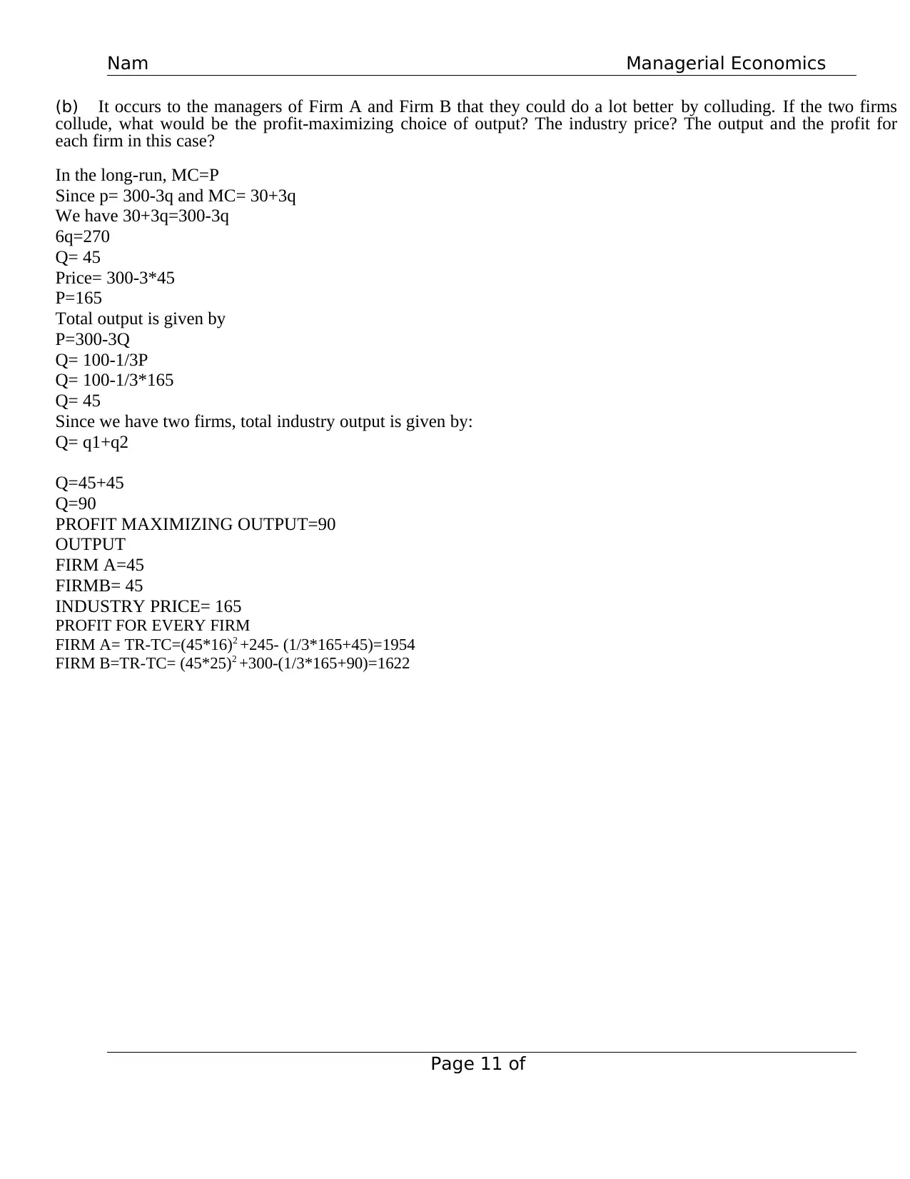
(b) It occurs to the managers of Firm A and Firm B that they could do a lot better by colluding. If the two firms
collude, what would be the profit-maximizing choice of output? The industry price? The output and the profit for
each firm in this case?
In the long-run, MC=P
Since p= 300-3q and MC= 30+3q
We have 30+3q=300-3q
6q=270
Q= 45
Price= 300-3*45
P=165
Total output is given by
P=300-3Q
Q= 100-1/3P
Q= 100-1/3*165
Q= 45
Since we have two firms, total industry output is given by:
Q= q1+q2
Q=45+45
Q=90
PROFIT MAXIMIZING OUTPUT=90
OUTPUT
FIRM A=45
FIRMB= 45
INDUSTRY PRICE= 165
PROFIT FOR EVERY FIRM
FIRM A= TR-TC=(45*16)2 +245- (1/3*165+45)=1954
FIRM B=TR-TC= (45*25)2 +300-(1/3*165+90)=1622
2009 H
Nam
e:
Page 11 of
15
(b) It occurs to the managers of Firm A and Firm B that they could do a lot better by colluding. If the two firms
collude, what would be the profit-maximizing choice of output? The industry price? The output and the profit for
each firm in this case?
In the long-run, MC=P
Since p= 300-3q and MC= 30+3q
We have 30+3q=300-3q
6q=270
Q= 45
Price= 300-3*45
P=165
Total output is given by
P=300-3Q
Q= 100-1/3P
Q= 100-1/3*165
Q= 45
Since we have two firms, total industry output is given by:
Q= q1+q2
Q=45+45
Q=90
PROFIT MAXIMIZING OUTPUT=90
OUTPUT
FIRM A=45
FIRMB= 45
INDUSTRY PRICE= 165
PROFIT FOR EVERY FIRM
FIRM A= TR-TC=(45*16)2 +245- (1/3*165+45)=1954
FIRM B=TR-TC= (45*25)2 +300-(1/3*165+90)=1622

Managerial Economics
2009 H
Nam
e:
Page 12 of
15
(c) The managers of these firms realize that explicit agreements to collude are illegal. Each firm must decide on its
own whether to produce the Cournot quantity or the cartel quantity. To aid in making the decision, the manager of
Firm A constructs a payoff matrix like the real one below. Fill in each box with the (profit of Firm A, profit of Firm
B). Given this payoff matrix, what output strategy is each firm likely to pursue?
Profit Payoff Matrix
Firm B
Produce Cournot q Produce Cartel Q
Produce Cournot q
Produce Cartel q
The firms are likely to pursue the third box where firm A earns 1954 while firm B earns 1622 because it yield the highest
income for both the firms. Firm
1540
1700
1622
1700
1540
1954
1622
1954
⊘ This is a preview!⊘
Do you want full access?
Subscribe today to unlock all pages.
Trusted by 1+ million students worldwide
1 out of 18
Related Documents


Your All-in-One AI-Powered Toolkit for Academic Success.
+13062052269
info@desklib.com
Available 24*7 on WhatsApp / Email
![[object Object]](/_next/static/media/star-bottom.7253800d.svg)
Unlock your academic potential
Copyright © 2020–2026 A2Z Services. All Rights Reserved. Developed and managed by ZUCOL.