AP Statistics: Empirical Validation of the Central Limit Theorem

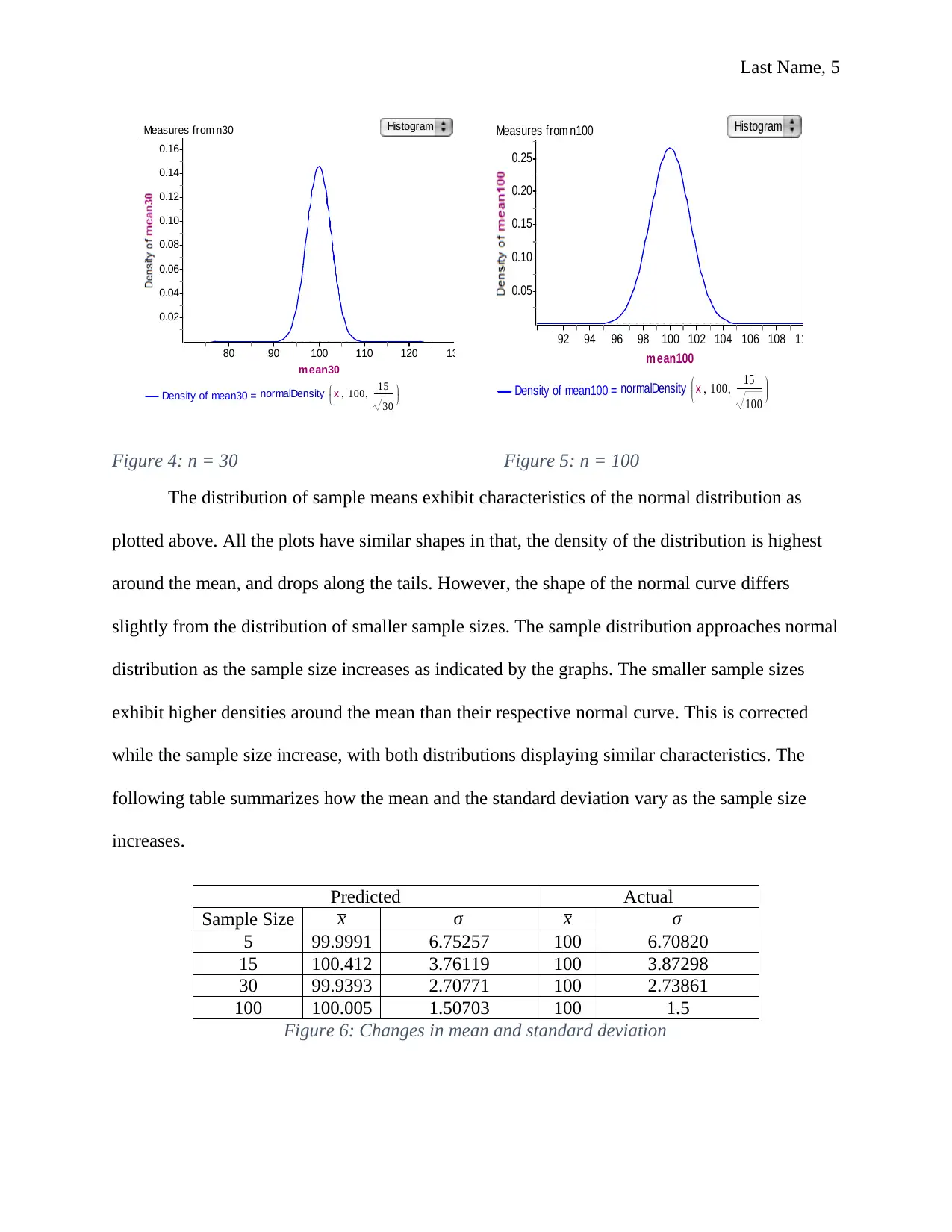
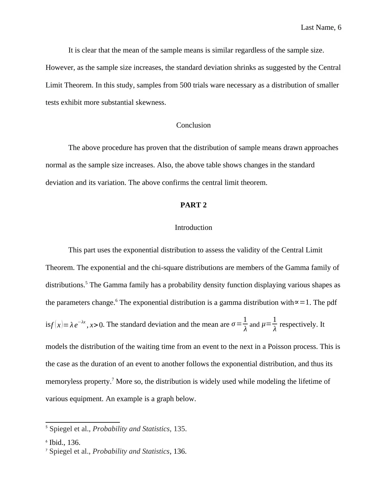
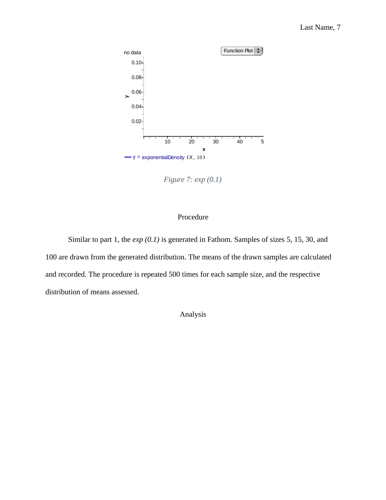
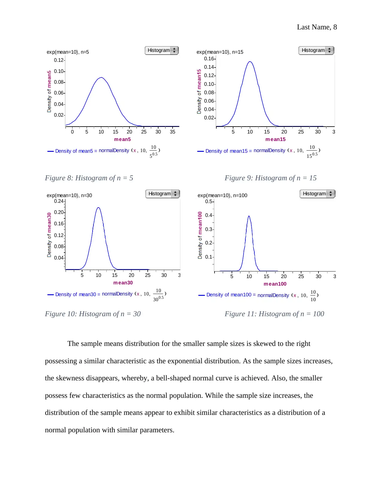
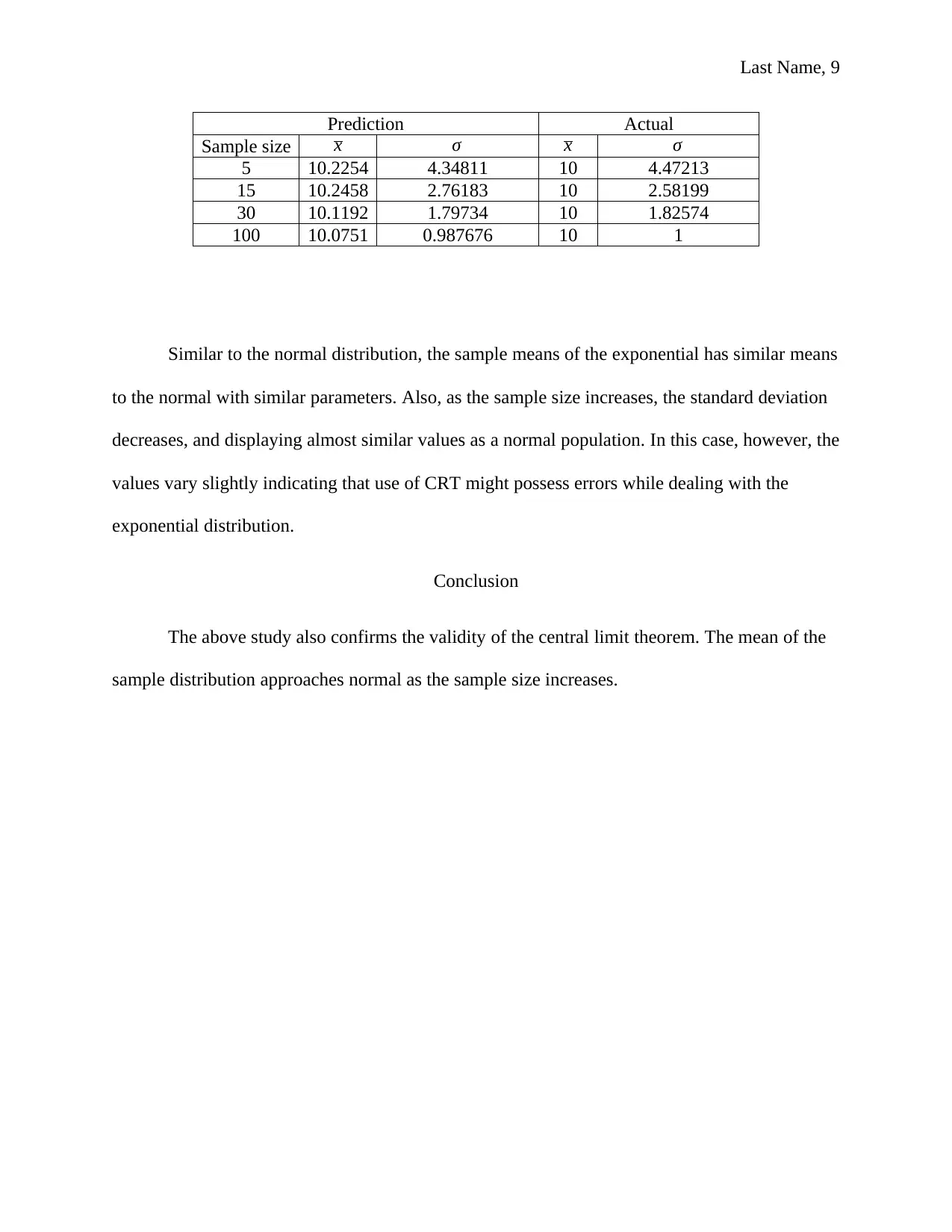
This report provides an empirical validation of the Central Limit Theorem (CLT) using both normal and exponential distributions. Part 1 focuses on the normal distribution, generating samples of varying sizes (n=5, 15, 30, 100) and analyzing the distribution of sample means using Fathom. The results demonstrate that as the sample size increases, the distribution of sample means approaches a normal distribution, confirming the CLT. Part 2 extends the analysis to the exponential distribution, known for its skewness, and repeats the sampling process. The findings indicate that even with a non-normal population, the distribution of sample means tends towards normality as the sample size grows, further supporting the CLT. The report includes detailed histograms, statistical measures, and comparisons between predicted and actual values to illustrate the convergence towards normality and the decrease in standard deviation with increasing sample size. The study concludes that the central limit theorem holds true and is valid.

The Central Limit Theorem
Name
AP Statistics
Instructor’s Name
Date

Last Name, 2
PART 1
Introduction
As one of the most important results in statistics, Central Limit Theorem gives a way of
inferencing large samples about the population mean, when the distribution of the population is
unknown, or doesn’t need to be known.1 More so, it provides inference about a population
proportion, example while conducting surveys. Further, it approximates the distribution of the
mean for any distribution, as well as approximating other distributions.2 In this study, we are
concerned about the approximation of the mean of various distributions.
The Central Limit Theorem states that, as n → ∞ for a sequence X1 , X2 , … , Xn of
identically, independently distributed random variables with finite mean and variance μ and
variance σ 2respectively, then, ´X−μ
σ / √n distribution approaches the standard normal distribution.
´X = 1
n ∑
i=1
n
Xi.3 The three properties of a sampling distribution are that it is normally distributed,
with mean μ, and standard deviation σ / √n . In Part 1, the validity of the theorem is going to be
assessed using the normal distribution, employing Fathom as a tool for the analysis.
Procedure
The normal distribution portrays a symmetrical (bell-shaped) density curve and is of
utmost importance while practicing, or in theoretical statistics. The distribution can be used
while modeling the distribution of student grades in a class; approximating other distributions,
1Walpole et al., Essentials of Probability and Statistics, 79.
2 Soong, Fundamentals of probability and statistics, 154.
3 Ibid., 154

Last Name, 3
example the limiting form of binomial ( n , θ ), Poisson ( μ ), among others; providing models for
sampling distributions of various statistics; while in statistical inference, most assumptions
regarding the underlying distribution are regarded as normal distribution; and acts as a building
block for other distributions, example the student’s t.4 The following graph shows the
distribution of a N (100, 15).
The normal distribution follows a probability density function defined asf ( x )= 1
σ √2 π e
−1
2 ( x−μ
σ )2
.
4 Chatfield, Statistics for technology, 89.
5
10
15
20
25
30
60 80 100 120 140 160
x
y = x    normalDensity
no data Function Plot
Figure 1: N (100, 15)

Last Name, 4
Samples of different sizes are generated from N (100, 15). The sample sizes drawn are 5,
15, 30, and 100. From each sample, the mean is calculated and recorded. Another sample of
similar size is pulled, the mean calculated and recorded. The procedure is repeated 500 times for
each sample size. Then, the distribution of sample means is evaluated as below.
Analysis
10
20
30
40
50
60
70
70 80 90 100 110 120 130
m ean5
Density of mean5 (thousandths) = x  

 
 
 normalDensity
Measures from n5 Histogram
0.02
0.04
0.06
0.08
0.10
0.12
70 80 90 100 110 120 130
m ean15
Density of mean15 = x  

 
 
 normalDensity
Measures from n15 Histogram
Figure 2: n = 5 Figure 3: n = 15

Last Name, 5
0.02
0.04
0.06
0.08
0.10
0.12
0.14
0.16
80 90 100 110 120 130
m ean30
Density of mean30 = x  

 
 
 normalDensity
Measures from n30 Histogram
0.05
0.10
0.15
0.20
0.25
92 94 96 98 100 102 104 106 108 110
m ean100
Density of mean100 = x  

 
 
 normalDensity
Measures from n100 Histogram
Figure 4: n = 30 Figure 5: n = 100
The distribution of sample means exhibit characteristics of the normal distribution as
plotted above. All the plots have similar shapes in that, the density of the distribution is highest
around the mean, and drops along the tails. However, the shape of the normal curve differs
slightly from the distribution of smaller sample sizes. The sample distribution approaches normal
distribution as the sample size increases as indicated by the graphs. The smaller sample sizes
exhibit higher densities around the mean than their respective normal curve. This is corrected
while the sample size increase, with both distributions displaying similar characteristics. The
following table summarizes how the mean and the standard deviation vary as the sample size
increases.
Predicted Actual
Sample Size x σ x σ
5 99.9991 6.75257 100 6.70820
15 100.412 3.76119 100 3.87298
30 99.9393 2.70771 100 2.73861
100 100.005 1.50703 100 1.5
Figure 6: Changes in mean and standard deviation

Last Name, 6
It is clear that the mean of the sample means is similar regardless of the sample size.
However, as the sample size increases, the standard deviation shrinks as suggested by the Central
Limit Theorem. In this study, samples from 500 trials ware necessary as a distribution of smaller
tests exhibit more substantial skewness.
Conclusion
The above procedure has proven that the distribution of sample means drawn approaches
normal as the sample size increases. Also, the above table shows changes in the standard
deviation and its variation. The above confirms the central limit theorem.
PART 2
Introduction
This part uses the exponential distribution to assess the validity of the Central Limit
Theorem. The exponential and the chi-square distributions are members of the Gamma family of
distributions.5 The Gamma family has a probability density function displaying various shapes as
the parameters change.6 The exponential distribution is a gamma distribution with∝=1. The pdf
is f ( x ) = λ e−λx , x> 0. The standard deviation and the mean are σ = 1
λ and μ= 1
λ respectively. It
models the distribution of the waiting time from an event to the next in a Poisson process. This is
the case as the duration of an event to another follows the exponential distribution, and thus its
memoryless property.7 More so, the distribution is widely used while modeling the lifetime of
various equipment. An example is a graph below.
5 Spiegel et al., Probability and Statistics, 135.
6 Ibid., 136.
7 Spiegel et al., Probability and Statistics, 136.

Last Name, 7
0.02
0.04
0.06
0.08
0.10
10 20 30 40 50
x
y = X  exponentialDensity
no data Function Plot
Figure 7: exp (0.1)
Procedure
Similar to part 1, the exp (0.1) is generated in Fathom. Samples of sizes 5, 15, 30, and
100 are drawn from the generated distribution. The means of the drawn samples are calculated
and recorded. The procedure is repeated 500 times for each sample size, and the respective
distribution of means assessed.
Analysis

Last Name, 8
0.02
0.04
0.06
0.08
0.10
0.12
0 5 10 15 20 25 30 35
m ean5
Density of mean5 = x  
 
  normalDensity
exp(mean=10), n=5 Histogram
0.02
0.04
0.06
0.08
0.10
0.12
0.14
0.16
5 10 15 20 25 30 35
m ean15
Density of mean15 = x  

  normalDensity
exp(mean=10), n=15 Histogram
Figure 8: Histogram of n = 5 Figure 9: Histogram of n = 15
0.04
0.08
0.12
0.16
0.20
0.24
5 10 15 20 25 30 35
m ean30
Density of mean30 = x  
 
  normalDensity
exp(mean=10), n=30 Histogram
0.1
0.2
0.3
0.4
0.5
5 10 15 20 25 30 35
m ean100
Density of mean100 = x  

  normalDensity
exp(mean=10), n=100 Histogram
Figure 10: Histogram of n = 30 Figure 11: Histogram of n = 100
The sample means distribution for the smaller sample sizes is skewed to the right
possessing a similar characteristic as the exponential distribution. As the sample sizes increases,
the skewness disappears, whereby, a bell-shaped normal curve is achieved. Also, the smaller
possess few characteristics as the normal population. While the sample size increases, the
distribution of the sample means appear to exhibit similar characteristics as a distribution of a
normal population with similar parameters.

Last Name, 9
Prediction Actual
Sample size x σ x σ
5 10.2254 4.34811 10 4.47213
15 10.2458 2.76183 10 2.58199
30 10.1192 1.79734 10 1.82574
100 10.0751 0.987676 10 1
Similar to the normal distribution, the sample means of the exponential has similar means
to the normal with similar parameters. Also, as the sample size increases, the standard deviation
decreases, and displaying almost similar values as a normal population. In this case, however, the
values vary slightly indicating that use of CRT might possess errors while dealing with the
exponential distribution.
Conclusion
The above study also confirms the validity of the central limit theorem. The mean of the
sample distribution approaches normal as the sample size increases.

Last Name, 10
Bibliography
Chatfield, Chris. Statistics for technology: a course in applied statistics. Routledge, 2018.
Soong, Tsu T. Fundamentals of probability and statistics for engineers. John Wiley &
Sons, 2004.
Spiegel, Murray R., John J. Schiller, and R. Srinivasan. Probability and statistics. New
York: McGraw-Hill,, 2013.
Walpole, Ronald E., Raymond H. Myers, Sharon L. Myers, and Keying Ye. Essentials of
Probability and Statistics for Engineers and Scientists. Pearson, 2014.