Applied Econometrics: Analysis of CEO Salaries and Firm Performance
VerifiedAdded on 2023/03/20
|18
|4047
|93
Report
AI Summary
This report applies econometric techniques to analyze CEO salaries, focusing on factors influencing compensation and firm performance. Task 1 utilizes multiple regression models to assess the impact of variables like return on equity, sales, and industry sectors on CEO salaries. The analysis includes hypothesis testing, such as ANOVA, to determine significant differences in salaries across sectors. Task 2 employs panel data estimators to analyze production functions, discussing the strengths and weaknesses of different estimators and comparing findings with theoretical predictions. The report includes literature reviews, research methodologies, and detailed interpretations of statistical results, such as p-values, R-squared, and tests for heteroskedasticity and multicollinearity. The report also explores percentage changes in CEO salaries over time using multiple regression models. The conclusion summarizes the key findings and implications of the econometric analysis.

Applied Econometrics
Paraphrase This Document
Need a fresh take? Get an instant paraphrase of this document with our AI Paraphraser

TABLE OF CONTENTS
INTRODUCTION...........................................................................................................................3
TASK 1............................................................................................................................................3
4. Findings...................................................................................................................................4
1. Estimating level of significance @ 5% pertaining to the salaries of two CEO operating in
different sector such as industrial and financial..........................................................................4
2. Assessing 3 multiple regression models to identify the factors that may explain the CEO
salary in 1990...............................................................................................................................5
3. Explaining percentage change in CEO salary over 1989-90 using 3 multiple regression
model...........................................................................................................................................9
4.................................................................................................................................................13
TASK 2..........................................................................................................................................14
a. Specifying and estimating production function using 3 different panel-data estimators.......14
b. Discussing strengths and weaknesses of each panel-data estimator......................................16
c. Identifying preferred estimator and comparing findings with theoretical predictions and
empirical findings......................................................................................................................16
d. Conclusion.............................................................................................................................17
REFERENCES..............................................................................................................................18
INTRODUCTION
Econometrics is the branch of economics that is highly concerned with the use of and
application of mathematical models in the context of concerned problem or issue. In the present
times, business units lay high level of emphasis on undertaking statistical methods or tools and
techniques for discovering suitable information from economic data set. The present report is
based on different case situations which will provide deeper insight about the manner in which
multiple regression and panel estimation model assists in evaluating the concerned data set.
TASK 1
1. Introduction
In the current times, CEO’s salary determination becomes the major issue which is facing
by the business units. At the time of appointing CEO, several aspects are considered by the
business unit such as skills, experience in the concerned field etc. Hence, this task will provide
deeper insight about the factors that have an influence on CEO’s salary determination. Further, it
also entails the manner in which regression as well as post-estimation tests assist in making
evaluation of hypotheses and thereby making decisions.
2. Literature review
According to the views of Bragaw and Misangyi (2017) high level of relationship takes
place between pay and performance of CEO. Moreover, the main motive of business unit is to
maximize the wealth of shareholders to a great extent. Hence, this is one of the main factors from
which aspect of CEO’s salary determination are highly influenced. On the other side, Hou, Priem
and Goranova (2017) benchmark is the major factors that closely impact the level of CEO
compensation. In other words, it can be depicted that salary or compensation of CEO is highly
competitive and in line with the offerings of similar companies. Further, investors’ confidence on
concerned CEO also has greater impact on the salary of CEO. Moreover, investors usually gives
priority to the CEO who maximizes their wealth and returns as well.
3. Research methodology
⊘ This is a preview!⊘
Do you want full access?
Subscribe today to unlock all pages.
Trusted by 1+ million students worldwide
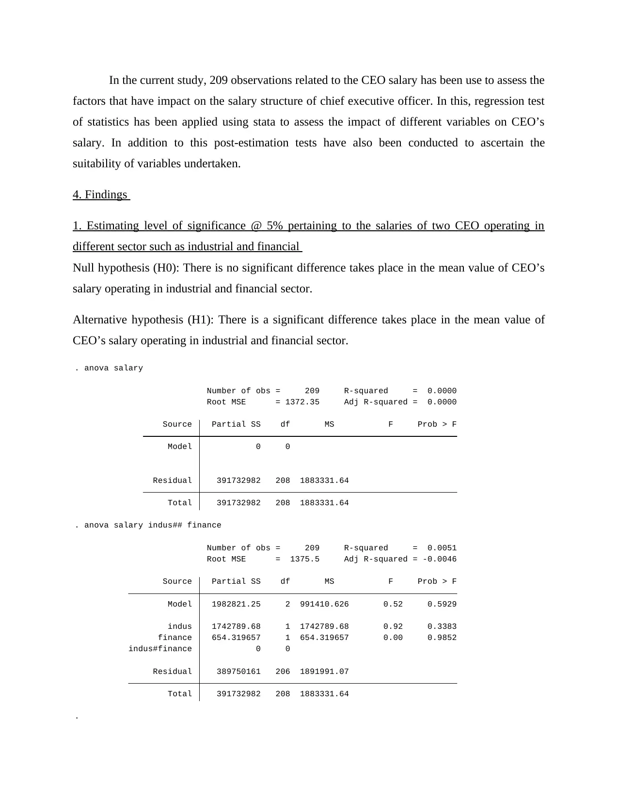
In the current study, 209 observations related to the CEO salary has been use to assess the
factors that have impact on the salary structure of chief executive officer. In this, regression test
of statistics has been applied using stata to assess the impact of different variables on CEO’s
salary. In addition to this post-estimation tests have also been conducted to ascertain the
suitability of variables undertaken.
4. Findings
1. Estimating level of significance @ 5% pertaining to the salaries of two CEO operating in
different sector such as industrial and financial
Null hypothesis (H0): There is no significant difference takes place in the mean value of CEO’s
salary operating in industrial and financial sector.
Alternative hypothesis (H1): There is a significant difference takes place in the mean value of
CEO’s salary operating in industrial and financial sector.
.
Total 391732982 208 1883331.64
Residual 389750161 206 1891991.07
indus#finance 0 0
finance 654.319657 1 654.319657 0.00 0.9852
indus 1742789.68 1 1742789.68 0.92 0.3383
Model 1982821.25 2 991410.626 0.52 0.5929
Source Partial SS df MS F Prob > F
Root MSE = 1375.5 Adj R-squared = -0.0046
Number of obs = 209 R-squared = 0.0051
. anova salary indus## finance
Total 391732982 208 1883331.64
Residual 391732982 208 1883331.64
Model 0 0
Source Partial SS df MS F Prob > F
Root MSE = 1372.35 Adj R-squared = 0.0000
Number of obs = 209 R-squared = 0.0000
. anova salary
Paraphrase This Document
Need a fresh take? Get an instant paraphrase of this document with our AI Paraphraser
Applying Two-way ANOVA test on data set, it has found that p value is greater than 0.05
in the context of both industrial and financial sector. By taking into such outcome, it can be
depicted that null hypothesis is accepted. In accordance with such aspect, salaries of CEO
working in industrial and financial sector are moving in the similar direction.
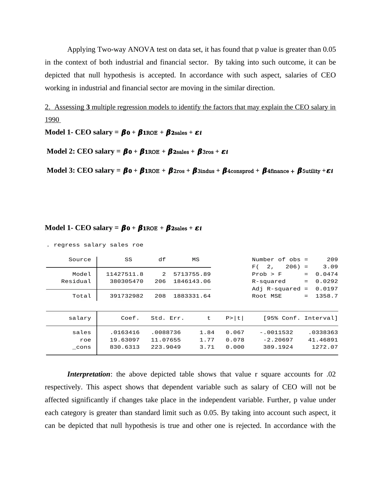
2. Assessing 3 multiple regression models to identify the factors that may explain the CEO salary in
1990
Model 1- CEO salary = 𝜷𝟎 + 𝜷𝟏ROE + 𝜷𝟐sales + 𝜺𝒊
Model 2: CEO salary = 𝜷𝟎 + 𝜷𝟏ROE + 𝜷𝟐sales + 𝜷3ros + 𝜺𝒊
Model 3: CEO salary = 𝜷𝟎 + 𝜷𝟏ROE + 𝜷2ros + 𝜷3indus + 𝜷4consprod + 𝜷4finance + 𝜷5utility +𝜺𝒊
Model 1- CEO salary = 𝜷𝟎 + 𝜷𝟏ROE + 𝜷𝟐sales + 𝜺𝒊
_cons 830.6313 223.9049 3.71 0.000 389.1924 1272.07
roe 19.63097 11.07655 1.77 0.078 -2.20697 41.46891
sales .0163416 .0088736 1.84 0.067 -.0011532 .0338363
salary Coef. Std. Err. t P>|t| [95% Conf. Interval]
Total 391732982 208 1883331.64 Root MSE = 1358.7
Adj R-squared = 0.0197
Residual 380305470 206 1846143.06 R-squared = 0.0292
Model 11427511.8 2 5713755.89 Prob > F = 0.0474
F( 2, 206) = 3.09
Source SS df MS Number of obs = 209
. regress salary sales roe
Interpretation: the above depicted table shows that value r square accounts for .02
respectively. This aspect shows that dependent variable such as salary of CEO will not be
affected significantly if changes take place in the independent variable. Further, p value under
each category is greater than standard limit such as 0.05. By taking into account such aspect, it
can be depicted that null hypothesis is true and other one is rejected. In accordance with the
in the context of both industrial and financial sector. By taking into such outcome, it can be
depicted that null hypothesis is accepted. In accordance with such aspect, salaries of CEO
working in industrial and financial sector are moving in the similar direction.
2. Assessing 3 multiple regression models to identify the factors that may explain the CEO salary in
1990
Model 1- CEO salary = 𝜷𝟎 + 𝜷𝟏ROE + 𝜷𝟐sales + 𝜺𝒊
Model 2: CEO salary = 𝜷𝟎 + 𝜷𝟏ROE + 𝜷𝟐sales + 𝜷3ros + 𝜺𝒊
Model 3: CEO salary = 𝜷𝟎 + 𝜷𝟏ROE + 𝜷2ros + 𝜷3indus + 𝜷4consprod + 𝜷4finance + 𝜷5utility +𝜺𝒊
Model 1- CEO salary = 𝜷𝟎 + 𝜷𝟏ROE + 𝜷𝟐sales + 𝜺𝒊
_cons 830.6313 223.9049 3.71 0.000 389.1924 1272.07
roe 19.63097 11.07655 1.77 0.078 -2.20697 41.46891
sales .0163416 .0088736 1.84 0.067 -.0011532 .0338363
salary Coef. Std. Err. t P>|t| [95% Conf. Interval]
Total 391732982 208 1883331.64 Root MSE = 1358.7
Adj R-squared = 0.0197
Residual 380305470 206 1846143.06 R-squared = 0.0292
Model 11427511.8 2 5713755.89 Prob > F = 0.0474
F( 2, 206) = 3.09
Source SS df MS Number of obs = 209
. regress salary sales roe
Interpretation: the above depicted table shows that value r square accounts for .02
respectively. This aspect shows that dependent variable such as salary of CEO will not be
affected significantly if changes take place in the independent variable. Further, p value under
each category is greater than standard limit such as 0.05. By taking into account such aspect, it
can be depicted that null hypothesis is true and other one is rejected. In accordance with the
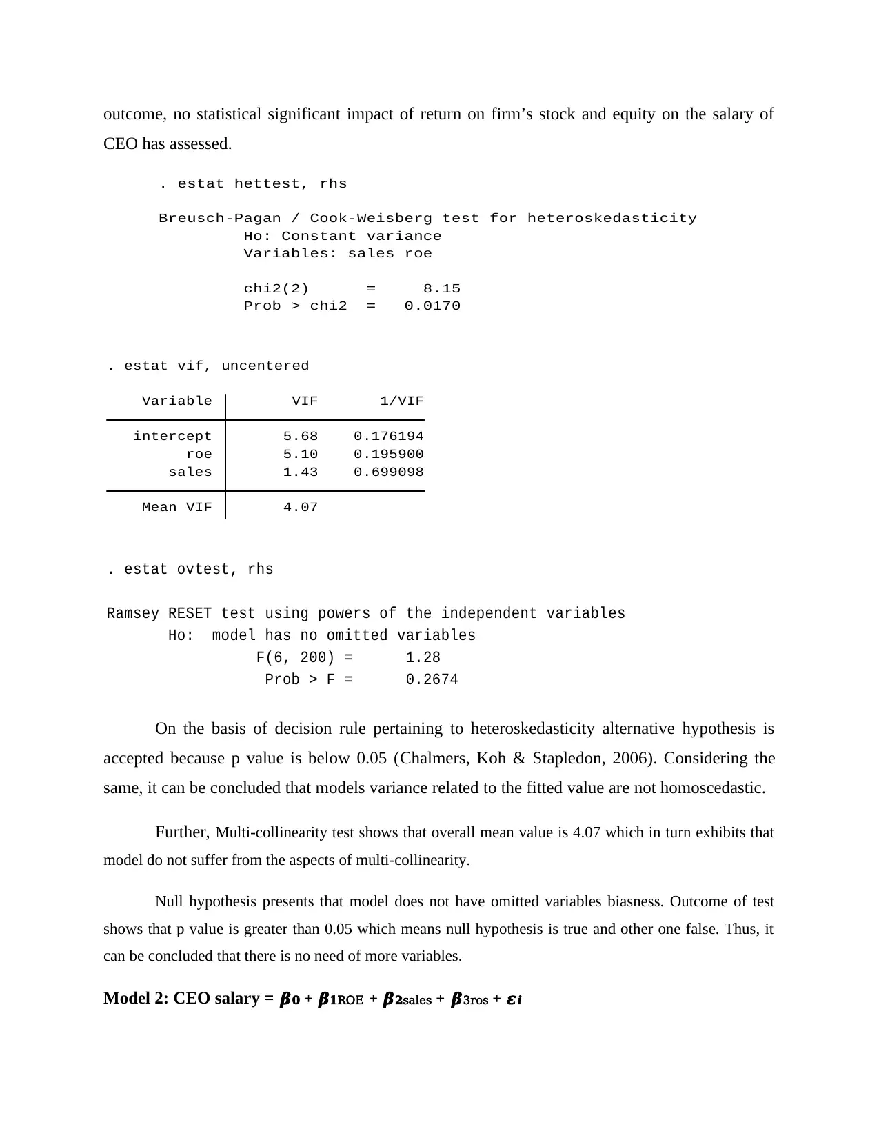
outcome, no statistical significant impact of return on firm’s stock and equity on the salary of
CEO has assessed.
Prob > chi2 = 0.0170
chi2(2) = 8.15
Variables: sales roe
Ho: Constant variance
Breusch-Pagan / Cook-Weisberg test for heteroskedasticity
. estat hettest, rhs
Mean VIF 4.07
sales 1.43 0.699098
roe 5.10 0.195900
intercept 5.68 0.176194
Variable VIF 1/VIF
. estat vif, uncentered
Prob > F = 0.2674
F(6, 200) = 1.28
Ho: model has no omitted variables
Ramsey RESET test using powers of the independent variables
. estat ovtest, rhs
On the basis of decision rule pertaining to heteroskedasticity alternative hypothesis is
accepted because p value is below 0.05 (Chalmers, Koh & Stapledon, 2006). Considering the
same, it can be concluded that models variance related to the fitted value are not homoscedastic.
Further, Multi-collinearity test shows that overall mean value is 4.07 which in turn exhibits that
model do not suffer from the aspects of multi-collinearity.
Null hypothesis presents that model does not have omitted variables biasness. Outcome of test
shows that p value is greater than 0.05 which means null hypothesis is true and other one false. Thus, it
can be concluded that there is no need of more variables.
Model 2: CEO salary = 𝜷𝟎 + 𝜷𝟏ROE + 𝜷𝟐sales + 𝜷3ros + 𝜺𝒊
⊘ This is a preview!⊘
Do you want full access?
Subscribe today to unlock all pages.
Trusted by 1+ million students worldwide
_cons 864.1175 228.3997 3.78 0.000 413.8038 1314.431
ros -1.105191 1.45024 -0.76 0.447 -3.96449 1.754108
sales .0154825 .0089539 1.73 0.085 -.0021711 .0331361
roe 22.00331 11.51655 1.91 0.057 -.7027663 44.70939
salary Coef. Std. Err. t P>|t| [95% Conf. Interval]
Total 391732982 208 1883331.64 Root MSE = 1360.1
Adj R-squared = 0.0177
Residual 379231123 205 1849907.92 R-squared = 0.0319
Model 12501859.4 3 4167286.46 Prob > F = 0.0834
F( 3, 205) = 2.25
Source SS df MS Number of obs = 209
. regress salary roe sales ros
Prob > chi2 = 0.0000
chi2(3) = 26.02
Variables: roe sales ros
Ho: Constant variance
Breusch-Pagan / Cook-Weisberg test for heteroskedasticity
. estat hettest, rhs
.
Mean VIF 3.72
sales 1.45 0.688017
ros 2.01 0.498304
roe 5.51 0.181587
intercept 5.89 0.169673
Variable VIF 1/VIF
. estat vif, uncentered
Prob > F = 0.5361
F(9, 196) = 0.89
Ho: model has no omitted variables
Ramsey RESET test using powers of the independent variables
. estat ovtest, rhs
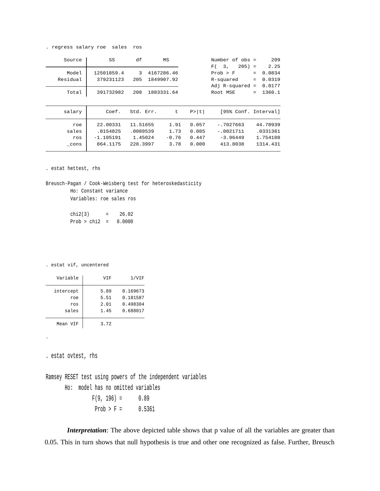
Interpretation: The above depicted table shows that p value of all the variables are greater than
0.05. This in turn shows that null hypothesis is true and other one recognized as false. Further, Breusch
ros -1.105191 1.45024 -0.76 0.447 -3.96449 1.754108
sales .0154825 .0089539 1.73 0.085 -.0021711 .0331361
roe 22.00331 11.51655 1.91 0.057 -.7027663 44.70939
salary Coef. Std. Err. t P>|t| [95% Conf. Interval]
Total 391732982 208 1883331.64 Root MSE = 1360.1
Adj R-squared = 0.0177
Residual 379231123 205 1849907.92 R-squared = 0.0319
Model 12501859.4 3 4167286.46 Prob > F = 0.0834
F( 3, 205) = 2.25
Source SS df MS Number of obs = 209
. regress salary roe sales ros
Prob > chi2 = 0.0000
chi2(3) = 26.02
Variables: roe sales ros
Ho: Constant variance
Breusch-Pagan / Cook-Weisberg test for heteroskedasticity
. estat hettest, rhs
.
Mean VIF 3.72
sales 1.45 0.688017
ros 2.01 0.498304
roe 5.51 0.181587
intercept 5.89 0.169673
Variable VIF 1/VIF
. estat vif, uncentered
Prob > F = 0.5361
F(9, 196) = 0.89
Ho: model has no omitted variables
Ramsey RESET test using powers of the independent variables
. estat ovtest, rhs
Interpretation: The above depicted table shows that p value of all the variables are greater than
0.05. This in turn shows that null hypothesis is true and other one recognized as false. Further, Breusch
Paraphrase This Document
Need a fresh take? Get an instant paraphrase of this document with our AI Paraphraser
Pagnan test model presents that p value is below the standard limit such as 0.05 which in turn shows that
alternative hypothesis is appropriate over null (Brick, Palmon & Wald, 2006). Mean as per multi-
collinearity test accounts for 3.72 significantly. This in turn exhibits that model does not suffering from
multi-collinearity. Ramsey test model shows that p>0.05 that means model does not suffer from any
errors.
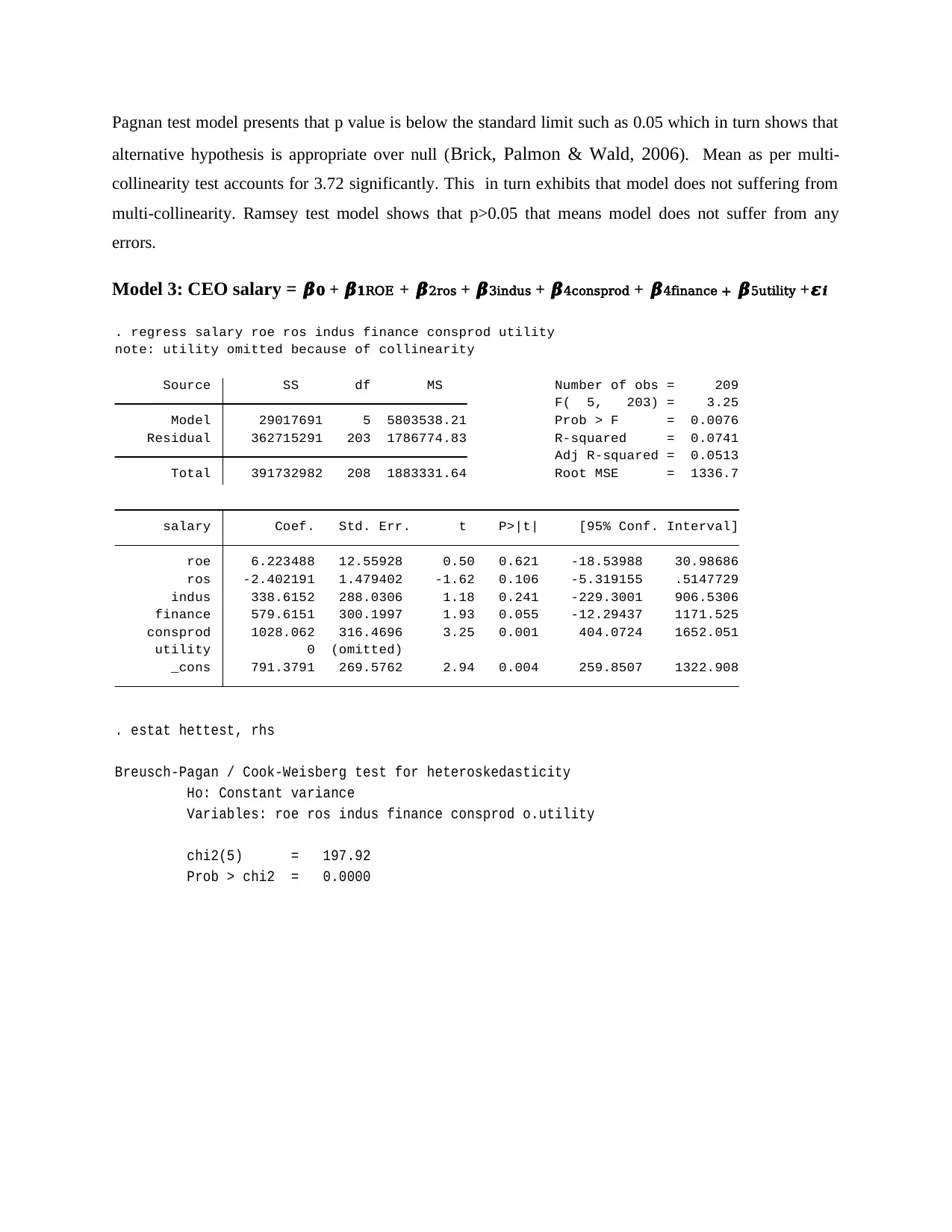
Model 3: CEO salary = 𝜷𝟎 + 𝜷𝟏ROE + 𝜷2ros + 𝜷3indus + 𝜷4consprod + 𝜷4finance + 𝜷5utility +𝜺𝒊
_cons 791.3791 269.5762 2.94 0.004 259.8507 1322.908
utility 0 (omitted)
consprod 1028.062 316.4696 3.25 0.001 404.0724 1652.051
finance 579.6151 300.1997 1.93 0.055 -12.29437 1171.525
indus 338.6152 288.0306 1.18 0.241 -229.3001 906.5306
ros -2.402191 1.479402 -1.62 0.106 -5.319155 .5147729
roe 6.223488 12.55928 0.50 0.621 -18.53988 30.98686
salary Coef. Std. Err. t P>|t| [95% Conf. Interval]
Total 391732982 208 1883331.64 Root MSE = 1336.7
Adj R-squared = 0.0513
Residual 362715291 203 1786774.83 R-squared = 0.0741
Model 29017691 5 5803538.21 Prob > F = 0.0076
F( 5, 203) = 3.25
Source SS df MS Number of obs = 209
note: utility omitted because of collinearity
. regress salary roe ros indus finance consprod utility
Prob > chi2 = 0.0000
chi2(5) = 197.92
Variables: roe ros indus finance consprod o.utility
Ho: Constant variance
Breusch-Pagan / Cook-Weisberg test for heteroskedasticity
. estat hettest, rhs
alternative hypothesis is appropriate over null (Brick, Palmon & Wald, 2006). Mean as per multi-
collinearity test accounts for 3.72 significantly. This in turn exhibits that model does not suffering from
multi-collinearity. Ramsey test model shows that p>0.05 that means model does not suffer from any
errors.
Model 3: CEO salary = 𝜷𝟎 + 𝜷𝟏ROE + 𝜷2ros + 𝜷3indus + 𝜷4consprod + 𝜷4finance + 𝜷5utility +𝜺𝒊
_cons 791.3791 269.5762 2.94 0.004 259.8507 1322.908
utility 0 (omitted)
consprod 1028.062 316.4696 3.25 0.001 404.0724 1652.051
finance 579.6151 300.1997 1.93 0.055 -12.29437 1171.525
indus 338.6152 288.0306 1.18 0.241 -229.3001 906.5306
ros -2.402191 1.479402 -1.62 0.106 -5.319155 .5147729
roe 6.223488 12.55928 0.50 0.621 -18.53988 30.98686
salary Coef. Std. Err. t P>|t| [95% Conf. Interval]
Total 391732982 208 1883331.64 Root MSE = 1336.7
Adj R-squared = 0.0513
Residual 362715291 203 1786774.83 R-squared = 0.0741
Model 29017691 5 5803538.21 Prob > F = 0.0076
F( 5, 203) = 3.25
Source SS df MS Number of obs = 209
note: utility omitted because of collinearity
. regress salary roe ros indus finance consprod utility
Prob > chi2 = 0.0000
chi2(5) = 197.92
Variables: roe ros indus finance consprod o.utility
Ho: Constant variance
Breusch-Pagan / Cook-Weisberg test for heteroskedasticity
. estat hettest, rhs
.
Mean VIF 4.37
ros 2.16 0.462511
finance 2.32 0.431014
indus 3.11 0.321453
consprod 3.36 0.297341
roe 6.78 0.147475
intercept 8.50 0.117641
Variable VIF 1/VIF
. estat vif, uncentered
Prob > F = 0.8999
F(6, 197) = 0.37
Ho: model has no omitted variables
Ramsey RESET test using powers of the independent variables
. estat ovtest, rhs
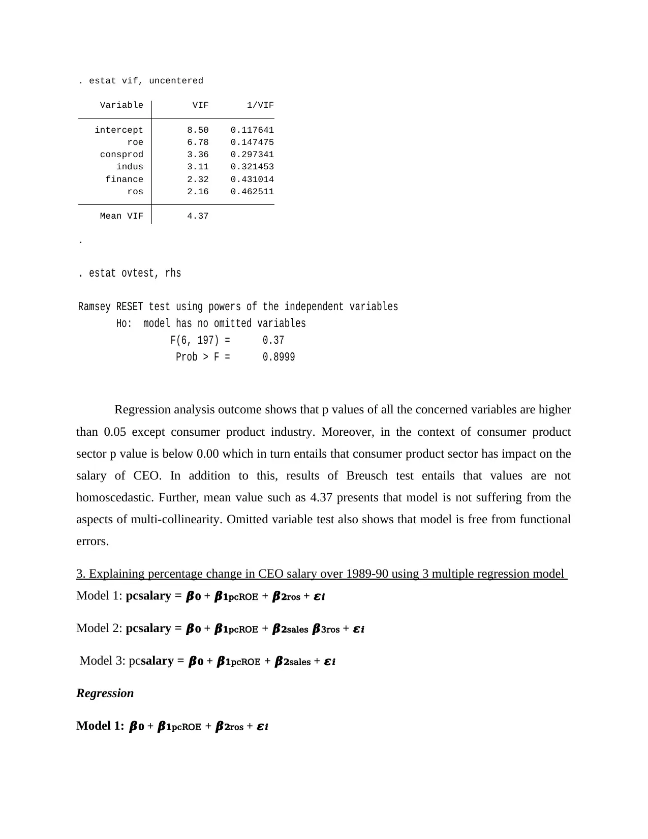
Regression analysis outcome shows that p values of all the concerned variables are higher
than 0.05 except consumer product industry. Moreover, in the context of consumer product
sector p value is below 0.00 which in turn entails that consumer product sector has impact on the
salary of CEO. In addition to this, results of Breusch test entails that values are not
homoscedastic. Further, mean value such as 4.37 presents that model is not suffering from the
aspects of multi-collinearity. Omitted variable test also shows that model is free from functional
errors.
3. Explaining percentage change in CEO salary over 1989-90 using 3 multiple regression model
Model 1: pcsalary = 𝜷𝟎 + 𝜷𝟏pcROE + 𝜷𝟐ros + 𝜺𝒊
Model 2: pcsalary = 𝜷𝟎 + 𝜷𝟏pcROE + 𝜷𝟐sales 𝜷3ros + 𝜺𝒊
Model 3: pcsalary = 𝜷𝟎 + 𝜷𝟏pcROE + 𝜷𝟐sales + 𝜺𝒊
Regression
Model 1: 𝜷𝟎 + 𝜷𝟏pcROE + 𝜷𝟐ros + 𝜺𝒊
Mean VIF 4.37
ros 2.16 0.462511
finance 2.32 0.431014
indus 3.11 0.321453
consprod 3.36 0.297341
roe 6.78 0.147475
intercept 8.50 0.117641
Variable VIF 1/VIF
. estat vif, uncentered
Prob > F = 0.8999
F(6, 197) = 0.37
Ho: model has no omitted variables
Ramsey RESET test using powers of the independent variables
. estat ovtest, rhs
Regression analysis outcome shows that p values of all the concerned variables are higher
than 0.05 except consumer product industry. Moreover, in the context of consumer product
sector p value is below 0.00 which in turn entails that consumer product sector has impact on the
salary of CEO. In addition to this, results of Breusch test entails that values are not
homoscedastic. Further, mean value such as 4.37 presents that model is not suffering from the
aspects of multi-collinearity. Omitted variable test also shows that model is free from functional
errors.
3. Explaining percentage change in CEO salary over 1989-90 using 3 multiple regression model
Model 1: pcsalary = 𝜷𝟎 + 𝜷𝟏pcROE + 𝜷𝟐ros + 𝜺𝒊
Model 2: pcsalary = 𝜷𝟎 + 𝜷𝟏pcROE + 𝜷𝟐sales 𝜷3ros + 𝜺𝒊
Model 3: pcsalary = 𝜷𝟎 + 𝜷𝟏pcROE + 𝜷𝟐sales + 𝜺𝒊
Regression
Model 1: 𝜷𝟎 + 𝜷𝟏pcROE + 𝜷𝟐ros + 𝜺𝒊
⊘ This is a preview!⊘
Do you want full access?
Subscribe today to unlock all pages.
Trusted by 1+ million students worldwide
_cons 9.242917 2.97821 3.10 0.002 3.371236 15.1146
ros .0540124 .0326796 1.65 0.100 -.0104169 .1184418
pcroe .0649234 .0229172 2.83 0.005 .019741 .1101058
pcsalary Coef. Std. Err. t P>|t| [95% Conf. Interval]
Total 221514.344 208 1064.97281 Root MSE = 31.864
Adj R-squared = 0.0466
Residual 209160.604 206 1015.34274 R-squared = 0.0558
Model 12353.7404 2 6176.87022 Prob > F = 0.0027
F( 2, 206) = 6.08
Source SS df MS Number of obs = 209
. regress pcsalary pcroe ros
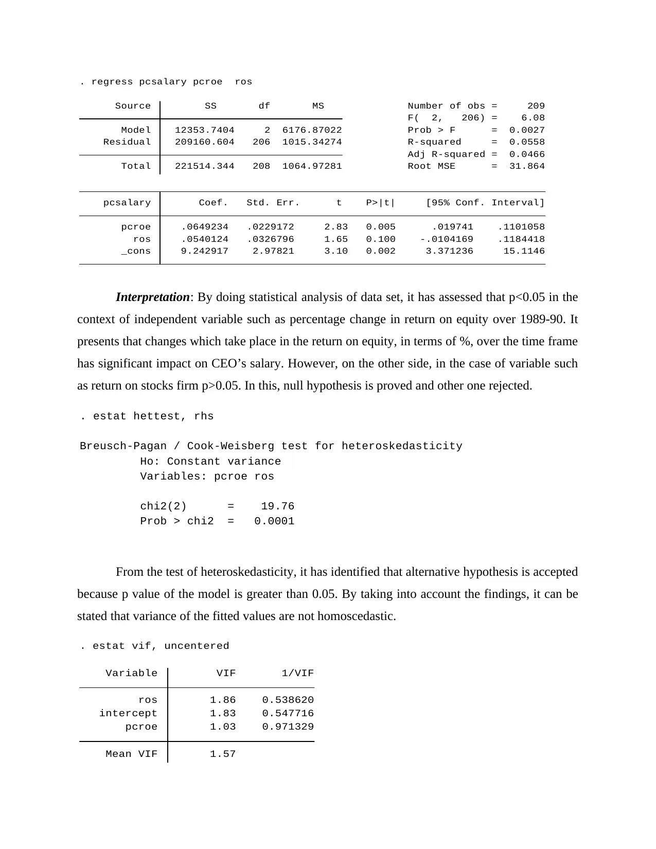
Interpretation: By doing statistical analysis of data set, it has assessed that p<0.05 in the
context of independent variable such as percentage change in return on equity over 1989-90. It
presents that changes which take place in the return on equity, in terms of %, over the time frame
has significant impact on CEO’s salary. However, on the other side, in the case of variable such
as return on stocks firm p>0.05. In this, null hypothesis is proved and other one rejected.
Prob > chi2 = 0.0001
chi2(2) = 19.76
Variables: pcroe ros
Ho: Constant variance
Breusch-Pagan / Cook-Weisberg test for heteroskedasticity
. estat hettest, rhs
From the test of heteroskedasticity, it has identified that alternative hypothesis is accepted
because p value of the model is greater than 0.05. By taking into account the findings, it can be
stated that variance of the fitted values are not homoscedastic.
Mean VIF 1.57
pcroe 1.03 0.971329
intercept 1.83 0.547716
ros 1.86 0.538620
Variable VIF 1/VIF
. estat vif, uncentered
ros .0540124 .0326796 1.65 0.100 -.0104169 .1184418
pcroe .0649234 .0229172 2.83 0.005 .019741 .1101058
pcsalary Coef. Std. Err. t P>|t| [95% Conf. Interval]
Total 221514.344 208 1064.97281 Root MSE = 31.864
Adj R-squared = 0.0466
Residual 209160.604 206 1015.34274 R-squared = 0.0558
Model 12353.7404 2 6176.87022 Prob > F = 0.0027
F( 2, 206) = 6.08
Source SS df MS Number of obs = 209
. regress pcsalary pcroe ros
Interpretation: By doing statistical analysis of data set, it has assessed that p<0.05 in the
context of independent variable such as percentage change in return on equity over 1989-90. It
presents that changes which take place in the return on equity, in terms of %, over the time frame
has significant impact on CEO’s salary. However, on the other side, in the case of variable such
as return on stocks firm p>0.05. In this, null hypothesis is proved and other one rejected.
Prob > chi2 = 0.0001
chi2(2) = 19.76
Variables: pcroe ros
Ho: Constant variance
Breusch-Pagan / Cook-Weisberg test for heteroskedasticity
. estat hettest, rhs
From the test of heteroskedasticity, it has identified that alternative hypothesis is accepted
because p value of the model is greater than 0.05. By taking into account the findings, it can be
stated that variance of the fitted values are not homoscedastic.
Mean VIF 1.57
pcroe 1.03 0.971329
intercept 1.83 0.547716
ros 1.86 0.538620
Variable VIF 1/VIF
. estat vif, uncentered
Paraphrase This Document
Need a fresh take? Get an instant paraphrase of this document with our AI Paraphraser
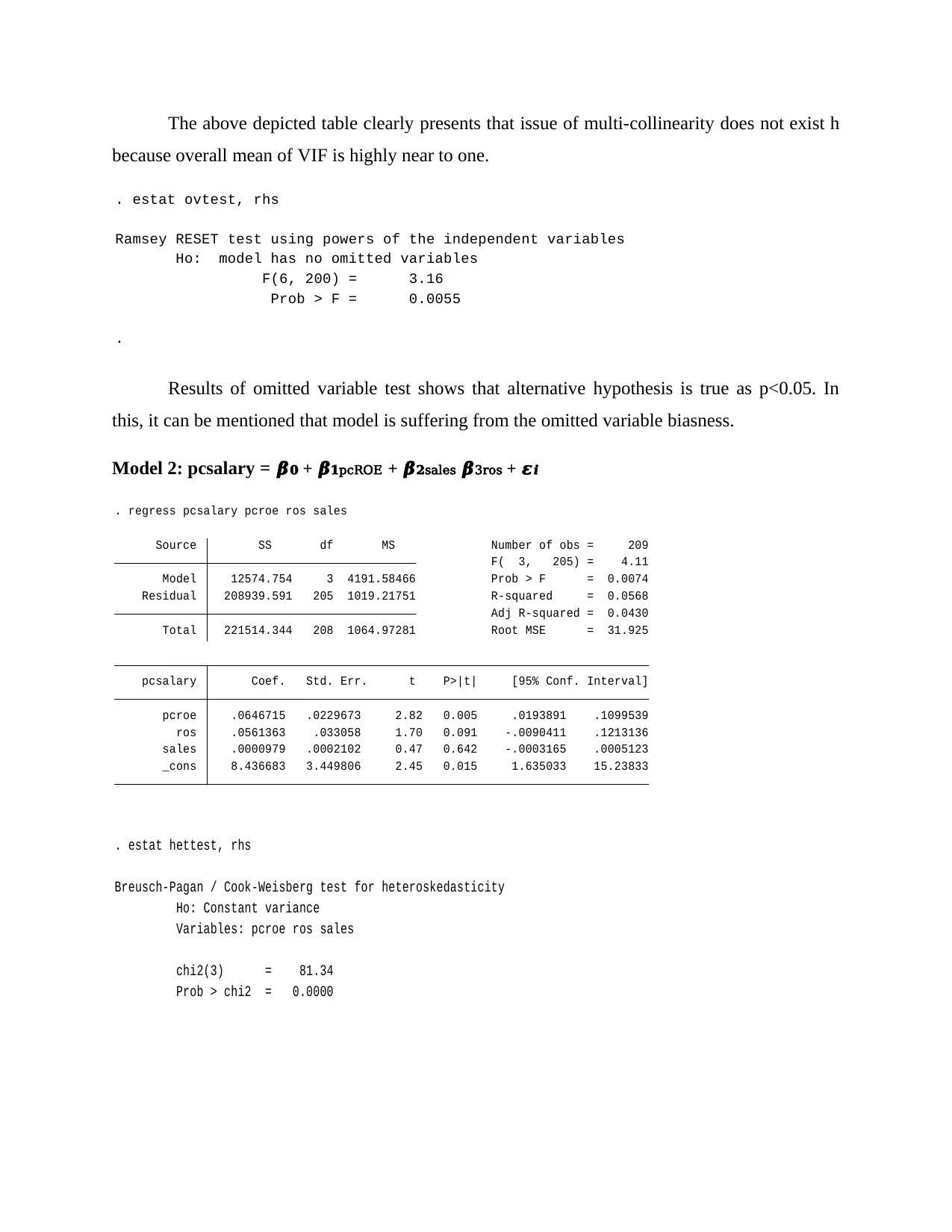
The above depicted table clearly presents that issue of multi-collinearity does not exist h
because overall mean of VIF is highly near to one.
.
Prob > F = 0.0055
F(6, 200) = 3.16
Ho: model has no omitted variables
Ramsey RESET test using powers of the independent variables
. estat ovtest, rhs
Results of omitted variable test shows that alternative hypothesis is true as p<0.05. In
this, it can be mentioned that model is suffering from the omitted variable biasness.
Model 2: pcsalary = 𝜷𝟎 + 𝜷𝟏pcROE + 𝜷𝟐sales 𝜷3ros + 𝜺𝒊
_cons 8.436683 3.449806 2.45 0.015 1.635033 15.23833
sales .0000979 .0002102 0.47 0.642 -.0003165 .0005123
ros .0561363 .033058 1.70 0.091 -.0090411 .1213136
pcroe .0646715 .0229673 2.82 0.005 .0193891 .1099539
pcsalary Coef. Std. Err. t P>|t| [95% Conf. Interval]
Total 221514.344 208 1064.97281 Root MSE = 31.925
Adj R-squared = 0.0430
Residual 208939.591 205 1019.21751 R-squared = 0.0568
Model 12574.754 3 4191.58466 Prob > F = 0.0074
F( 3, 205) = 4.11
Source SS df MS Number of obs = 209
. regress pcsalary pcroe ros sales
Prob > chi2 = 0.0000
chi2(3) = 81.34
Variables: pcroe ros sales
Ho: Constant variance
Breusch-Pagan / Cook-Weisberg test for heteroskedasticity
. estat hettest, rhs
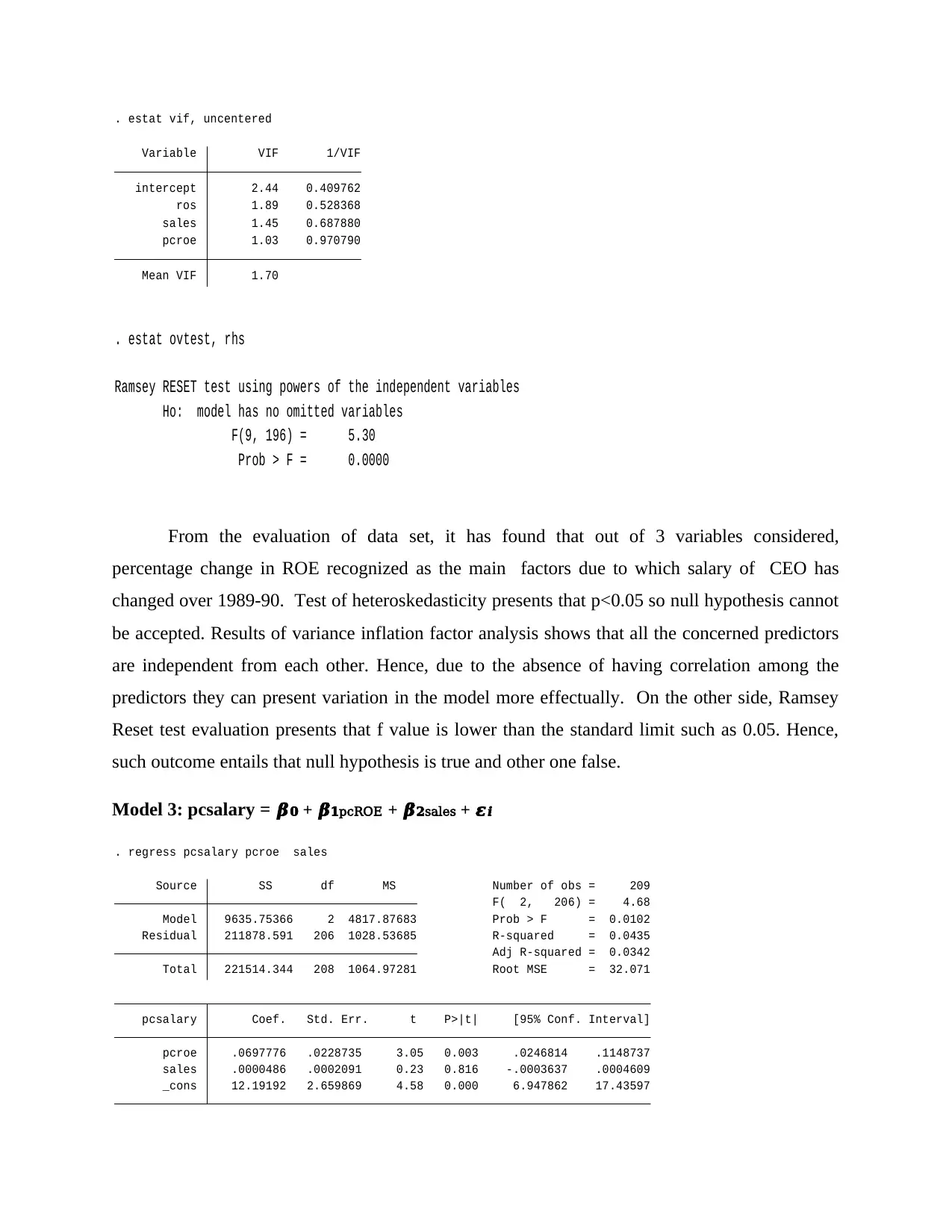
Mean VIF 1.70
pcroe 1.03 0.970790
sales 1.45 0.687880
ros 1.89 0.528368
intercept 2.44 0.409762
Variable VIF 1/VIF
. estat vif, uncentered
Prob > F = 0.0000
F(9, 196) = 5.30
Ho: model has no omitted variables
Ramsey RESET test using powers of the independent variables
. estat ovtest, rhs
From the evaluation of data set, it has found that out of 3 variables considered,
percentage change in ROE recognized as the main factors due to which salary of CEO has
changed over 1989-90. Test of heteroskedasticity presents that p<0.05 so null hypothesis cannot
be accepted. Results of variance inflation factor analysis shows that all the concerned predictors
are independent from each other. Hence, due to the absence of having correlation among the
predictors they can present variation in the model more effectually. On the other side, Ramsey
Reset test evaluation presents that f value is lower than the standard limit such as 0.05. Hence,
such outcome entails that null hypothesis is true and other one false.
Model 3: pcsalary = 𝜷𝟎 + 𝜷𝟏pcROE + 𝜷𝟐sales + 𝜺𝒊
_cons 12.19192 2.659869 4.58 0.000 6.947862 17.43597
sales .0000486 .0002091 0.23 0.816 -.0003637 .0004609
pcroe .0697776 .0228735 3.05 0.003 .0246814 .1148737
pcsalary Coef. Std. Err. t P>|t| [95% Conf. Interval]
Total 221514.344 208 1064.97281 Root MSE = 32.071
Adj R-squared = 0.0342
Residual 211878.591 206 1028.53685 R-squared = 0.0435
Model 9635.75366 2 4817.87683 Prob > F = 0.0102
F( 2, 206) = 4.68
Source SS df MS Number of obs = 209
. regress pcsalary pcroe sales
⊘ This is a preview!⊘
Do you want full access?
Subscribe today to unlock all pages.
Trusted by 1+ million students worldwide
1 out of 18
Related Documents


Your All-in-One AI-Powered Toolkit for Academic Success.
+13062052269
info@desklib.com
Available 24*7 on WhatsApp / Email
![[object Object]](/_next/static/media/star-bottom.7253800d.svg)
Unlock your academic potential
Copyright © 2020–2026 A2Z Services. All Rights Reserved. Developed and managed by ZUCOL.