CFD Analysis: Fluid Flow in Rectangular Pipe and Vehicle Models

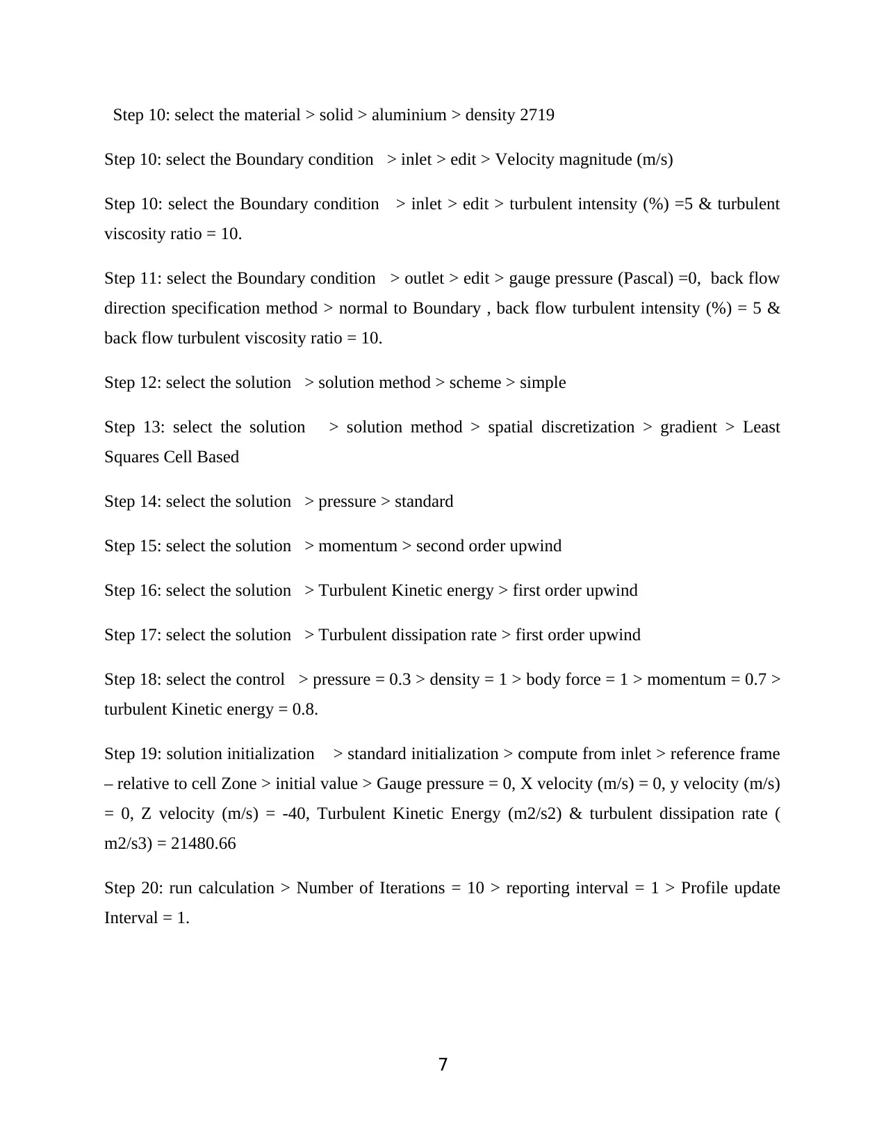
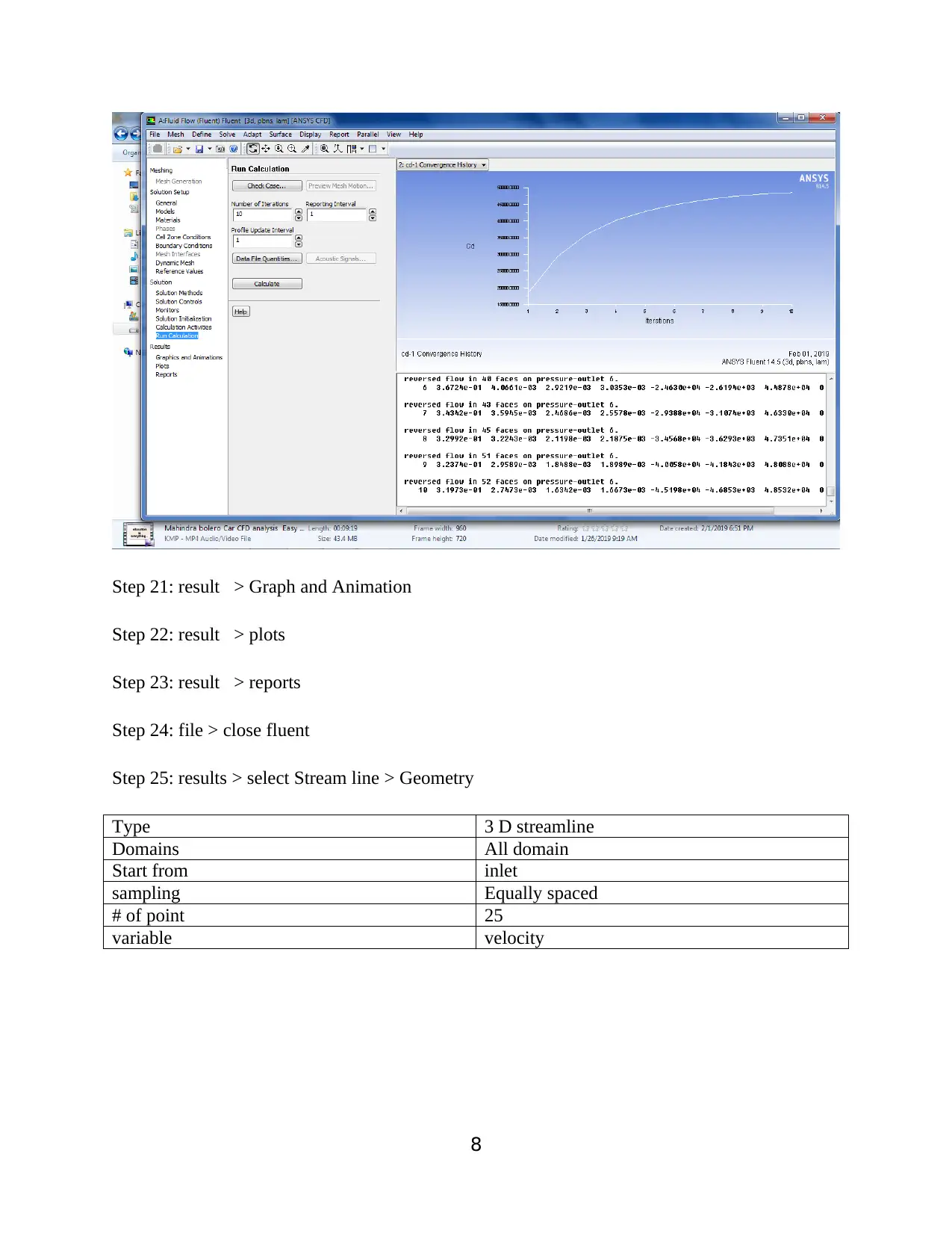
This report presents a comprehensive CFD (Computational Fluid Dynamics) analysis, focusing on fluid flow simulations in various engineering applications. It begins with an overview of the objectives, including the comparison of fluid velocity and pressure in rectangular pipes, and the visualization of streamline and contour flows. The introduction covers CFD applications in civil, environmental, and naval engineering, particularly in the context of automobile and engine design. The methodology section details the step-by-step procedure using ANSYS software, including CAD model creation, mesh settings, boundary conditions, and solution methods. The report also discusses the finite element method and spectral method, comparing their approaches to solving partial differential equations. Furthermore, it covers the application of CFD in creating vehicle models, with and without spoilers, and outlines the process of meshing the model for accurate simulation results. The report also includes a discussion on the advantages and disadvantages of CFD, along with references for further reading.

CFD
[Document subtitle]
MARCH 13, 2018
HP
[Company address]

Contents
General Information...........................................................................................................................................0
1. The objective of the simulation:- Main objective of CFD analysis is following.......................................0
2. Introduction to CFD...................................................................................................................................0
3. CFD in Automobile and Engine Applications...........................................................................................0
Methodology......................................................................................................................................................1
Procedure..........................................................................................................................................................11
Finite Element Method.....................................................................................................................................11
Spectral method................................................................................................................................................12
Application of CFD..........................................................................................................................................13
Application of Ansyse software.......................................................................................................................13
Advantage of CFD:..........................................................................................................................................17
Disadvantage of CFD:......................................................................................................................................17
Review..............................................................................................................................................................17
References........................................................................................................................................................18
II

General Information
1. The objective of the simulation:- Main objective of CFD analysis is following
a. Comparison of inlet and outlet velocity of fluid in Rectangular pipe.
b. Comparison of inlet and outlet presser of fluid in Rectangular pipe.
c. To show the streamline flow in Rectangular pipe in different position like fluid, solid, or
all domain.
d. To show the Contour flow in Rectangular pipe
e. To show the Velocity vector in Rectangular pipe
f. To produce a standard computational fluid dynamics simulation of a vehicle model and to
withdraw relevant data’s.
g. To produce standard of CFD simulations result of drag phenomenon to two cars that are
following eachother. (A., 1996)
2. Introduction to CFD:-
 Civil Engineering Applications: - Rehology of rivers, estuaries, lakes etc. problems are
also the major subject the need to be investigated through CFD. One of the example is the
pumping of mud from an underwater mud capture reservoir. Here, a layer of water sits on
top of a layer of mud, and portion of mud is trapped and is being sucked away at the
bottom. CFD is capable of calculating the velocity field of both mud and water at any
instant
 Environmental Engineering Applications:- CFD gets involved while designing the
building in accordance the heating, air conditioning and general air circulation.
 Naval Architecture Applications-Submarine: - CFD acts as a major source to solve the
hydrodynamic problems that gets encounter with ships, submarines, etc. (K.J., 2001)
3. CFD in Automobile and Engine Applications.
Automobile industries has thrown its hat in the research field associated with the high technology
inordewr to improve the performance of their vehicles. For the same context, they are employing

CFD for the better conceptions of the flow processes and improving the design with the better
substitute. (Bhise, 2017)
Methodology
Step1. Make the 3d Module in the Cad software (Creo, Catia, Solid work, Unigraphix, or any
another cad software) according to given dimension then it convert into .IGS or .STP file.
Step 2. Start the workbench of the ansys software
Step3. Select the module
Example.
 Design as assessment
 Electric
 Explicit dynamic
 Fluid flow – blow molding (poly flow)
 Fluid flow – extrusion (poly flow)
 Fluid flow (CFX)
 Fluid flow (fluent)
 Fluid flow (poly flow)
 Harmonic response
 Hydrodynamic diffraction
 Hydrodynamic time response
 IC engine
 Linear Buckling
 Magnetostatic
 Modal
 Modal (samcef)
 Random vibration
 Response spectrum
 Rigid dynamics
 Static structural
1

 Static structural (samcef)
 Steady- state thermal
 Thermal electric
 Through flow
 Transient structural
 Transient thermal
Component systems
 Autodyne
 Blade gen
 CFX
 Engineering data
 Explicitly dynamic
 External connection
 External data
 Finite element modeller
 Fluent
 Fluent ( with T Grid meshing)
 Geometry
 ICEM CFD
 Icepak
 Mechanical APDL
 Mechanical Model
 Mesh
 Microsoft office excel
 Poly flow
 Poly flow – Blow Molding
 Poly flow – Extrusion
 Result
 System Coupling
 Turbo grid
2

 Vista AFD
 Vista CCD
 Vista CCD (with CCM)
 Vista CPD
 Vista RTD
 Vista TF
Custom systems
 FSI: Fluid Flow(CFX)
 FSI: Fluid Flow(Fluent)
 Pre Stress Modal
 Random Vibration
 Response Spectrum
 Thermal stress
Design Exploration
 Direct optimization
 Parameters correlation
 Response surface
 Response surface optimization
 Six sigma analysis
Step 4. Select Fluid flow fluent (for this project)
3

Step 5 : select the Geometry as shown in fig. then import the Geometry > generate the
Geometry . fill the geometry inside the rectangular pipe (as a fluid)
Step 6: close the design modeller
Step 7: select the Mesh
 Setting the mesh > defaults
Physics CFD
Solver preference Fluent
relevance 100
 Setting the mesh > select the sizing
Use advance size function On curvature
Relevance centre fine
Initial size seed Active assembly
Smoothing High
Transition slow
Span angle centre Fine
Curvature normal angle Default(12)
Min size Default (6.0027e-00m)
Max face size Default (0.600270m)
Max size Default (1.200050m)
Growth rate Default(1.10)
4

Minimum edge length 0.80 m
 Setting the mesh > inflation
 Setting the mesh > assembly meshing
 Setting the mesh > patch conforming option
 Setting the mesh > advance
 Setting the mesh > defeaturing
 Setting the mesh > statics
Step 7: generate the mesh
Step 7: select the setup
5

Step 8: select the general
Step 10: select the material > Fluid > Air > Density (kg/m^3) = 1.2 & viscosity (Kg/m-s) =
1.81e-005.
6

Step 10: select the material > solid > aluminium > density 2719
Step 10: select the Boundary condition > inlet > edit > Velocity magnitude (m/s)
Step 10: select the Boundary condition > inlet > edit > turbulent intensity (%) =5 & turbulent
viscosity ratio = 10.
Step 11: select the Boundary condition > outlet > edit > gauge pressure (Pascal) =0, back flow
direction specification method > normal to Boundary , back flow turbulent intensity (%) = 5 &
back flow turbulent viscosity ratio = 10.
Step 12: select the solution > solution method > scheme > simple
Step 13: select the solution > solution method > spatial discretization > gradient > Least
Squares Cell Based
Step 14: select the solution > pressure > standard
Step 15: select the solution > momentum > second order upwind
Step 16: select the solution > Turbulent Kinetic energy > first order upwind
Step 17: select the solution > Turbulent dissipation rate > first order upwind
Step 18: select the control > pressure = 0.3 > density = 1 > body force = 1 > momentum = 0.7 >
turbulent Kinetic energy = 0.8.
Step 19: solution initialization > standard initialization > compute from inlet > reference frame
– relative to cell Zone > initial value > Gauge pressure = 0, X velocity (m/s) = 0, y velocity (m/s)
= 0, Z velocity (m/s) = -40, Turbulent Kinetic Energy (m2/s2) & turbulent dissipation rate (
m2/s3) = 21480.66
Step 20: run calculation > Number of Iterations = 10 > reporting interval = 1 > Profile update
Interval = 1.
7

Step 21: result > Graph and Animation
Step 22: result > plots
Step 23: result > reports
Step 24: file > close fluent
Step 25: results > select Stream line > Geometry
Type 3 D streamline
Domains All domain
Start from inlet
sampling Equally spaced
# of point 25
variable velocity
8

Step 26: results > contour > Geometry
Domains All domain
location Contact region src
variable velocity
range Global
Colour scale linear
Colour Map Default (Rainbow)
Turbulence
9