STA2300 Statistics 2 Assignment 3, S2 2018: Data Analysis of CGD Study

This document provides a complete solution to a Statistics 2 assignment, focusing on data analysis from a Chronic Granulomatous Disease (CGD) study. The assignment involves using SPSS to calculate sample statistics, construct confidence intervals for the mean diastolic blood pressure, and perform hypothesis tests. The solution includes checking assumptions, calculating test statistics, determining p-values, and drawing conclusions based on the statistical results. The assignment covers topics such as one-sample mean tests, proportion tests, and paired t-tests, demonstrating the application of statistical methods to real-world data. The solution also addresses sample size calculations and interpretation of statistical outputs.

STATISTICS 2, 2018 1
STA2300 DATA ANALYSIS S2, 2018
[Name of Student]
[Institutional Affiliation]
[Date of Submission]
Assignment 3

STATISTICS 2, 2018 2
Question One
This sample data set has been adapted from a subset of data collected from a study of Gamma
Interferon in Chronic Granulomatous Disease (CGD).
You should use SPSS to calculate the sample statistics you will need to do this question, but for
the confidence interval in part (a) and test statistic in part (d) you are required to do the rest of
the calculations by hand, using a calculator.
(a) Using SPSS find the estimate of the Mean of population and SD of Diastolic BP of the
patients at beginning of the study (DBP_1). Find a 99% confidence interval for the mean
population Diastolic BP of the population of patients at the beginning of the study by
hand (show all working).
SPSS output of estimate of population mean and SD of Diastolic BP of the patients at the
beginning of the study (DBP_1).
Descriptive Statistics
N Mean Std. Deviation
DBP_1 170 84.69 13.019
Valid N (listwise) 170
Table 1: Estimate of population mean and SD of Diastolic BP of Patients at the beginning of
the study (DBP_1)
We then determine/construct the 99% confidence interval for the mean population Diastolic BP
of the population of patients at the beginning of the study (one-sample mean);
ӯ = 84.69
n = 170
s = 13.019
df (degrees of freedom)= n-1 = 169
Then t *(99%) = 2.576 from the given study table.
Both ӯ and S were obtained using SPSS as shown in the table 1 above (As stated in the
question).

STATISTICS 2, 2018 3
Thus the 99% confidence interval is constructed and obtained by;
95% CI = ӯ ± t*× s
√ n
= 84.69 ± 2.576 × 13.019
√ 170
= 84.69 ± 2.5722
Hence the 1% level of significance (99% confidence interval) for the mean population Diastolic
BP of the population of patients at the beginning of the study is 82.1178 to 87.2622
(b) Check the appropriate conditions and assumptions needed for the validity of the
confidence interval or hypothesis test for the population mean Diastolic BP of the
patients at the beginning of the study. Include graphical illustration in support of your
answer.
Checking the conditions and assumptions for the validity of the confidence interval or
hypothesis test for the population mean Diastolic BP of the patients at the beginning of the
study;
 Independence assumption; It is reasonable to assume that the population of Diastolic BP
patients is independent since we have a random sample.
 Random Sampling; we assume that we have a random sample as stated in the dataset (It
was a random sample from the normal distribution).
 Independency; It is assumed that the mean Diastolic BP of the patients at the beginning
of the study are independent of the Diastolic patients at the end of the study.
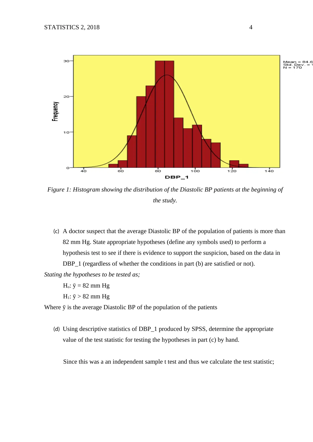
 Nearly condition of the normality; it is assumed that the distribution of the Diastolic BP
of the patients for the groups is normal. Also, the size of the sample n is relative bigger
for the theory of the central limit to be applied and the sampling distributions of the
sample mean will each be the normal model. The histogram below show that both the
groups have approximately symmetrical distribution.

STATISTICS 2, 2018 4
Figure 1: Histogram showing the distribution of the Diastolic BP patients at the beginning of
the study.
(c) A doctor suspect that the average Diastolic BP of the population of patients is more than
82 mm Hg. State appropriate hypotheses (define any symbols used) to perform a
hypothesis test to see if there is evidence to support the suspicion, based on the data in
DBP_1 (regardless of whether the conditions in part (b) are satisfied or not).
Stating the hypotheses to be tested as;
Ho: ӯ = 82 mm Hg
H1: ӯ > 82 mm Hg
Where ӯ is the average Diastolic BP of the population of the patients
(d) Using descriptive statistics of DBP_1 produced by SPSS, determine the appropriate
value of the test statistic for testing the hypotheses in part (c) by hand.
Since this was a an independent sample t test and thus we calculate the test statistic;

STATISTICS 2, 2018 5
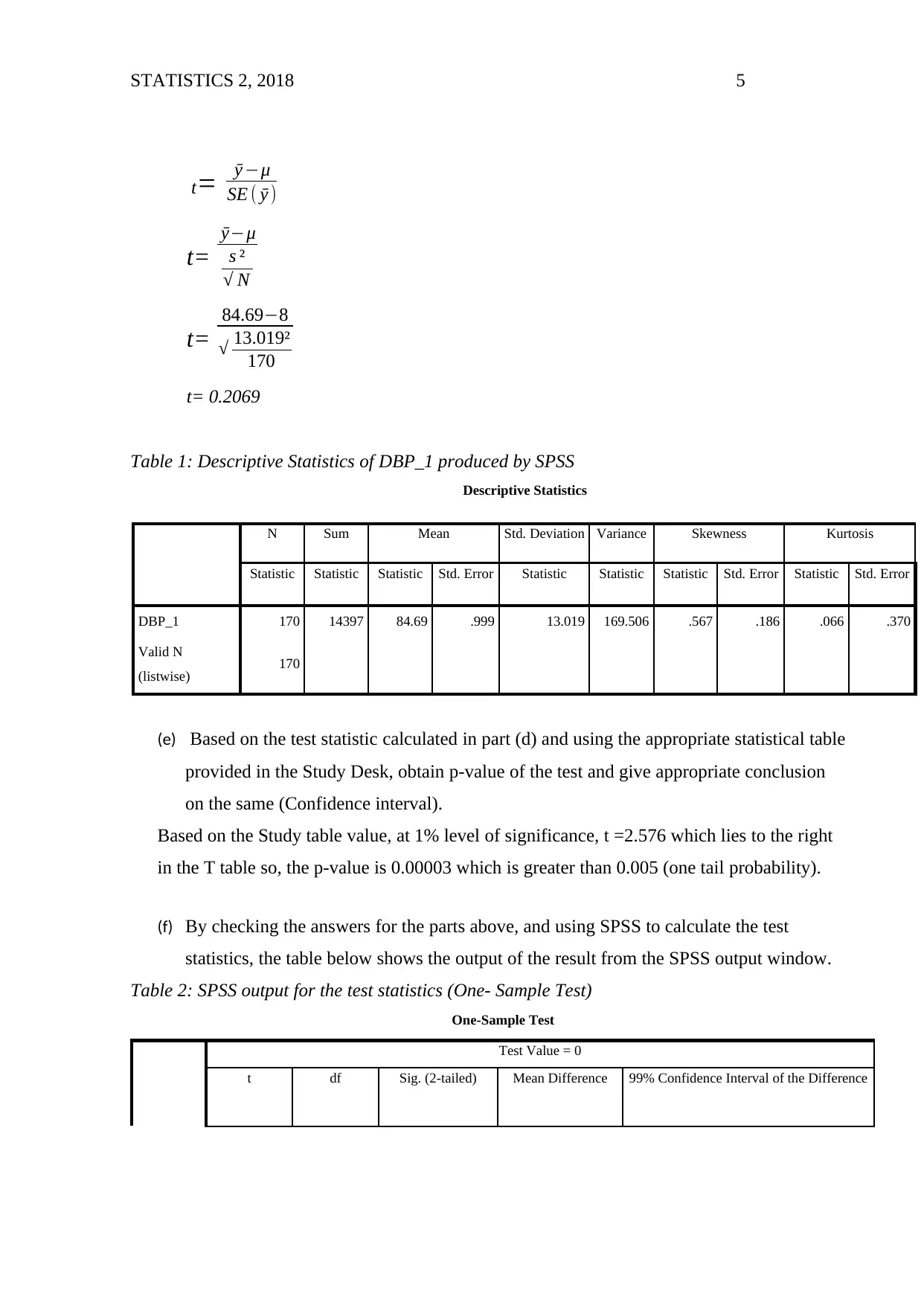
t= ӯ −μ
SE ( ӯ )
t=
ӯ−μ
s ²
√ N
t=
84.69−8
√ 13.019²
170
t= 0.2069
Table 1: Descriptive Statistics of DBP_1 produced by SPSS
Descriptive Statistics
N Sum Mean Std. Deviation Variance Skewness Kurtosis
Statistic Statistic Statistic Std. Error Statistic Statistic Statistic Std. Error Statistic Std. Error
DBP_1 170 14397 84.69 .999 13.019 169.506 .567 .186 .066 .370
Valid N
(listwise) 170
(e) Based on the test statistic calculated in part (d) and using the appropriate statistical table
provided in the Study Desk, obtain p-value of the test and give appropriate conclusion
on the same (Confidence interval).
Based on the Study table value, at 1% level of significance, t =2.576 which lies to the right
in the T table so, the p-value is 0.00003 which is greater than 0.005 (one tail probability).
(f) By checking the answers for the parts above, and using SPSS to calculate the test
statistics, the table below shows the output of the result from the SPSS output window.
Table 2: SPSS output for the test statistics (One- Sample Test)
One-Sample Test
Test Value = 0
t df Sig. (2-tailed) Mean Difference 99% Confidence Interval of the Difference

STATISTICS 2, 2018 6
Lower Upper
DBP_1 84.812 169 .000 84.688 82.09 87.29
In comparison with the calculated value, the difference is due to the existence of the standard
error term which is not inclusive in the calculated value. The error margin is not given based on
the SPSS output result while the error term is obtained when calculated manually (Not rounded
off or truncated).
Question Two
Considering the dataset cgd.sav is a random sample of all patients of a population answer the
following questions. You should use SPSS to calculate any sample statistics you will need to do
this question, but for parts (d)-(g) you are required to do the rest of the work by hand.
From previous studies it was known that the proportion of women patient suffering from the
disease was 0.25. A doctor claims that the proportion of women patient suffering from the
disease has changed in recent time.
(a) What is the variable of interest here?
The variable of interest here is the women patient suffering from the disease
(b) State the appropriate hypotheses (define any symbols used) to test the doctor’s claim
Stating the hypothesis to be tested as;
Ho: The Population of women patient suffering from the disease has not increased in
time
H1: The Population of women patient suffering from the disease has increased in time
OR (Symbolically stated as)
Ho: p = 0.25
H1: p ˂ 0.25
Where p = is the proportion of women suffering from the disease.

STATISTICS 2, 2018 7
(c) To test the hypothesis under consideration, we should first check the following
conditions and assumptions are met;
i. Random sampling; in relation to this assumption, it was clearly stated
that it was a random sample data of the patients from a population.
ii. The independence assumption; it would be reasonable to assume that the
proportion of women patient suffering from the disease was independent
and that the same proportion of the women patient suffering from the
disease has increased in the recent time.
iii. The 10% condition; in the absence of the information about the whole
population, we would assume that there are more than 170 women
patients. This also seems to be reasonable.
iv. The thumb rule; in regard to this assumption, both the np = 170 × 0.25 =
42.5 and n (1-p) = 170 (1-0.25) = 127.5 are all greater than 10 hence the
success of failure condition is also met.
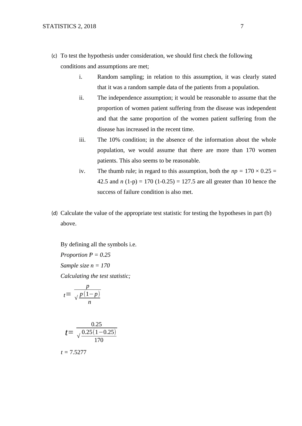
(d) Calculate the value of the appropriate test statistic for testing the hypotheses in part (b)
above.
By defining all the symbols i.e.
Proportion Ᵽ = 0.25
Sample size n = 170
Calculating the test statistic;
t=
p
√ p (1− p)
n
t=
0.25
√ 0.25(1−0.25)
170
t = 7.5277

STATISTICS 2, 2018 8
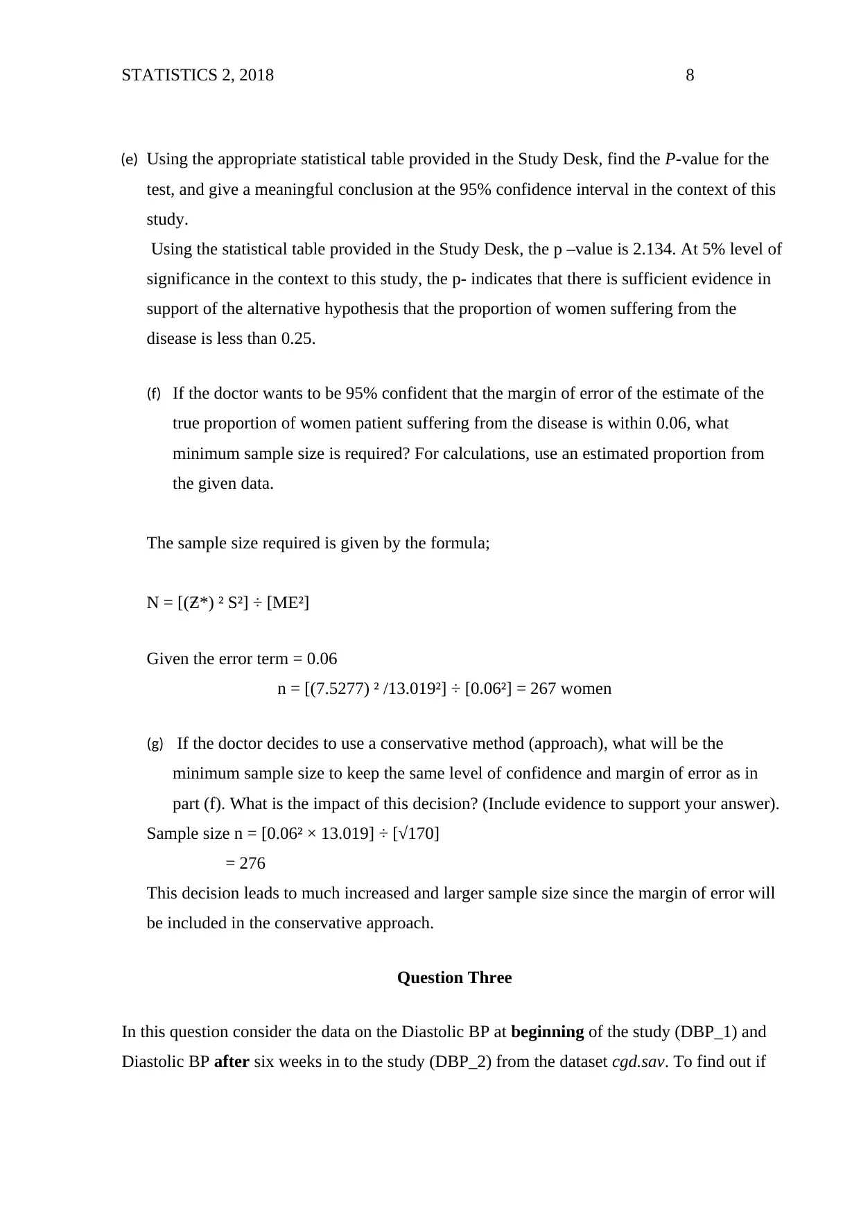
(e) Using the appropriate statistical table provided in the Study Desk, find the P-value for the
test, and give a meaningful conclusion at the 95% confidence interval in the context of this
study.
Using the statistical table provided in the Study Desk, the p –value is 2.134. At 5% level of
significance in the context to this study, the p- indicates that there is sufficient evidence in
support of the alternative hypothesis that the proportion of women suffering from the
disease is less than 0.25.
(f) If the doctor wants to be 95% confident that the margin of error of the estimate of the
true proportion of women patient suffering from the disease is within 0.06, what
minimum sample size is required? For calculations, use an estimated proportion from
the given data.
The sample size required is given by the formula;
N = [(Ƶ*) ² S²] ÷ [ME²]
Given the error term = 0.06
n = [(7.5277) ² /13.019²] ÷ [0.06²] = 267 women
(g) If the doctor decides to use a conservative method (approach), what will be the
minimum sample size to keep the same level of confidence and margin of error as in
part (f). What is the impact of this decision? (Include evidence to support your answer).
Sample size n = [0.06² × 13.019] ÷ [√170]
= 276
This decision leads to much increased and larger sample size since the margin of error will
be included in the conservative approach.
Question Three
In this question consider the data on the Diastolic BP at beginning of the study (DBP_1) and
Diastolic BP after six weeks in to the study (DBP_2) from the dataset cgd.sav. To find out if

STATISTICS 2, 2018 9
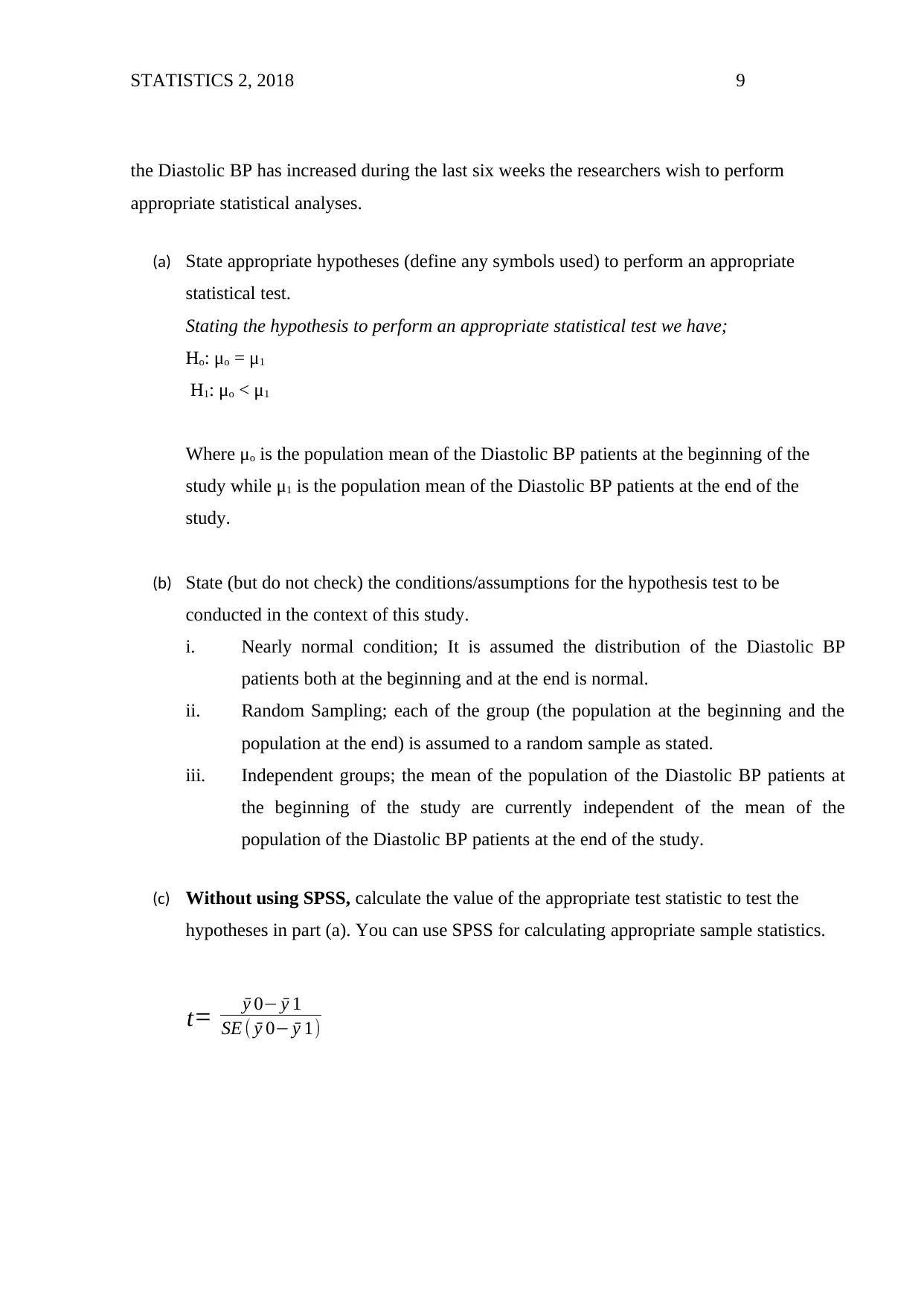
the Diastolic BP has increased during the last six weeks the researchers wish to perform
appropriate statistical analyses.
(a) State appropriate hypotheses (define any symbols used) to perform an appropriate
statistical test.
Stating the hypothesis to perform an appropriate statistical test we have;
Ho: μo = μ1
H1: μo ˂ μ1
Where μo is the population mean of the Diastolic BP patients at the beginning of the
study while μ1 is the population mean of the Diastolic BP patients at the end of the
study.
(b) State (but do not check) the conditions/assumptions for the hypothesis test to be
conducted in the context of this study.
i. Nearly normal condition; It is assumed the distribution of the Diastolic BP
patients both at the beginning and at the end is normal.
ii. Random Sampling; each of the group (the population at the beginning and the
population at the end) is assumed to a random sample as stated.
iii. Independent groups; the mean of the population of the Diastolic BP patients at
the beginning of the study are currently independent of the mean of the
population of the Diastolic BP patients at the end of the study.
(c) Without using SPSS, calculate the value of the appropriate test statistic to test the
hypotheses in part (a). You can use SPSS for calculating appropriate sample statistics.
t= ӯ 0− ӯ 1
SE ( ӯ 0− ӯ 1)

STATISTICS 2, 2018 10
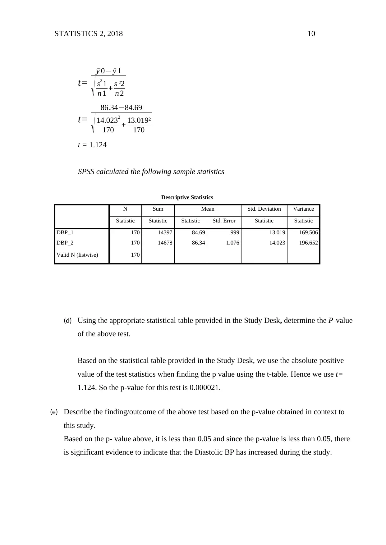
t=
ӯ 0− ӯ 1
√ s2 1
n 1 + s ²2
n 2
t=
86.34−84.69
√ 14.0232
170 + 13.019²
170
t = 1.124
SPSS calculated the following sample statistics
Descriptive Statistics
N Sum Mean Std. Deviation Variance
Statistic Statistic Statistic Std. Error Statistic Statistic
DBP_1 170 14397 84.69 .999 13.019 169.506
DBP_2 170 14678 86.34 1.076 14.023 196.652
Valid N (listwise) 170
(d) Using the appropriate statistical table provided in the Study Desk, determine the P-value
of the above test.
Based on the statistical table provided in the Study Desk, we use the absolute positive
value of the test statistics when finding the p value using the t-table. Hence we use t=
1.124. So the p-value for this test is 0.000021.
(e) Describe the finding/outcome of the above test based on the p-value obtained in context to
this study.
Based on the p- value above, it is less than 0.05 and since the p-value is less than 0.05, there
is significant evidence to indicate that the Diastolic BP has increased during the study.

STATISTICS 2, 2018 11
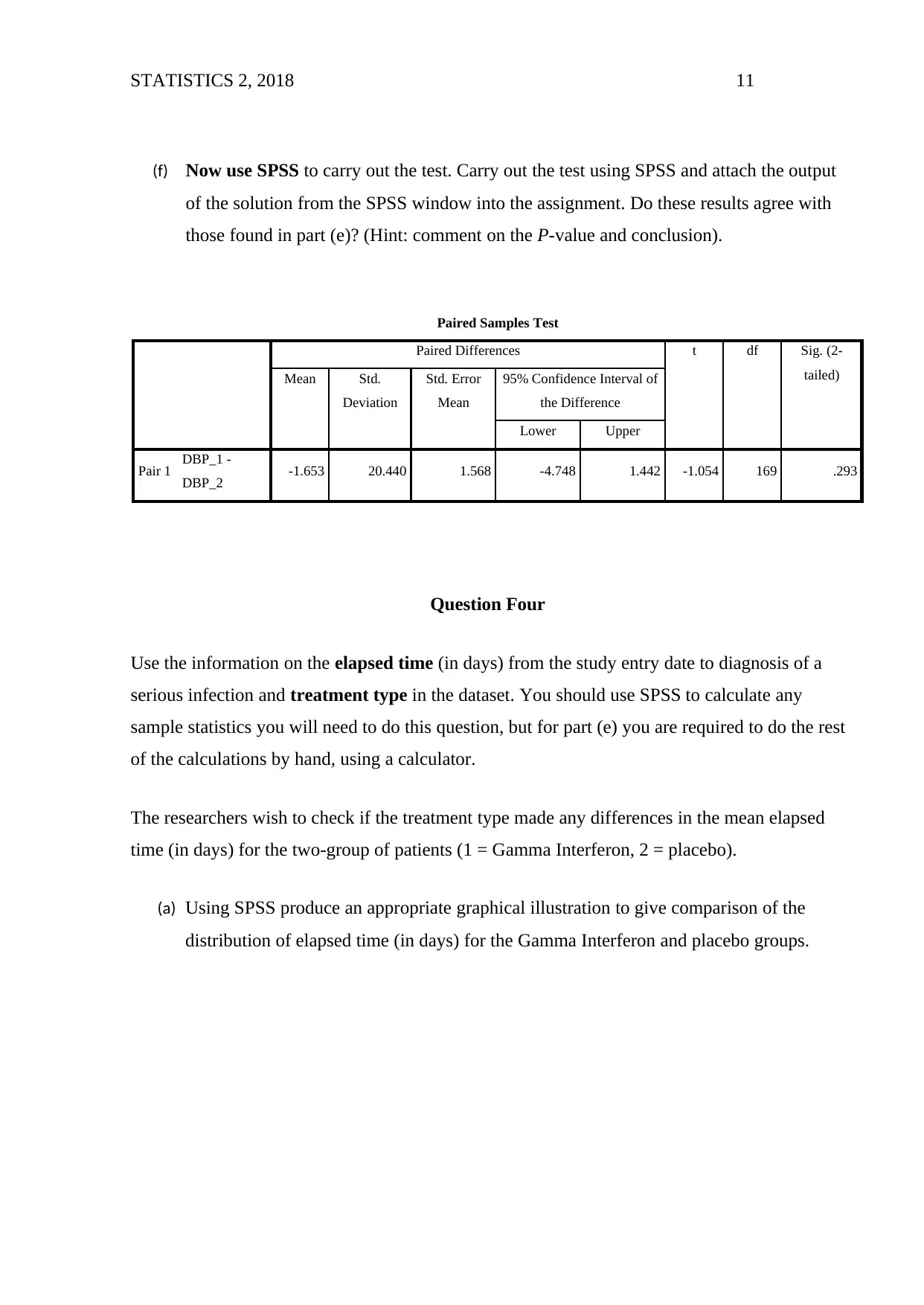
(f) Now use SPSS to carry out the test. Carry out the test using SPSS and attach the output
of the solution from the SPSS window into the assignment. Do these results agree with
those found in part (e)? (Hint: comment on the P-value and conclusion).
Paired Samples Test
Paired Differences t df Sig. (2-
tailed)Mean Std.
Deviation
Std. Error
Mean
95% Confidence Interval of
the Difference
Lower Upper
Pair 1 DBP_1 -
DBP_2 -1.653 20.440 1.568 -4.748 1.442 -1.054 169 .293
Question Four
Use the information on the elapsed time (in days) from the study entry date to diagnosis of a
serious infection and treatment type in the dataset. You should use SPSS to calculate any
sample statistics you will need to do this question, but for part (e) you are required to do the rest
of the calculations by hand, using a calculator.
The researchers wish to check if the treatment type made any differences in the mean elapsed
time (in days) for the two-group of patients (1 = Gamma Interferon, 2 = placebo).
(a) Using SPSS produce an appropriate graphical illustration to give comparison of the
distribution of elapsed time (in days) for the Gamma Interferon and placebo groups.

STATISTICS 2, 2018 12
Figure 4: Box plot of elapsed time for the Gamma and Interferon and placebo groups
(b) Using the graph produced in part (a), briefly describe the distribution of elapsed time for
the two groups of patients.
Based on the graph above, it is evident that there is normality in the distribution of elapsed
time for the two groups of patients. No outliers exist in the data.
(c) State appropriate hypotheses (defining all symbols) to answer the question: ‘Is the mean
elapsed time different for the two-group of patients?’
Ho: μo = μ1
H1: μo ≠ μ1
Where μo is the mean elapsed time for the Gamma Interferon while μ1 is the mean elapsed time
for the placebo
(d) Checking the requirements/assumptions for the validity of the test in relation to the
above part (c).
For us to test the hypothesis above, the following assumptions must be checked for the test
to be valid;
i. The distribution of the difference between Gamma Interferon and placebo over time
is normally distributed since the sample size is enough for the central limit theorem
to be applied.
ii. Random sample; the 170 are randomly selected from the population as stated.