University Chemistry Homework: Statistical Analysis and Calibration

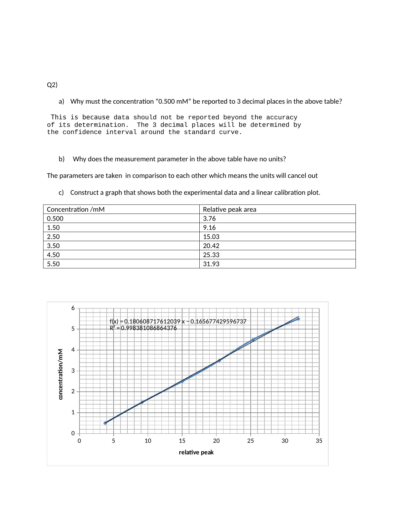
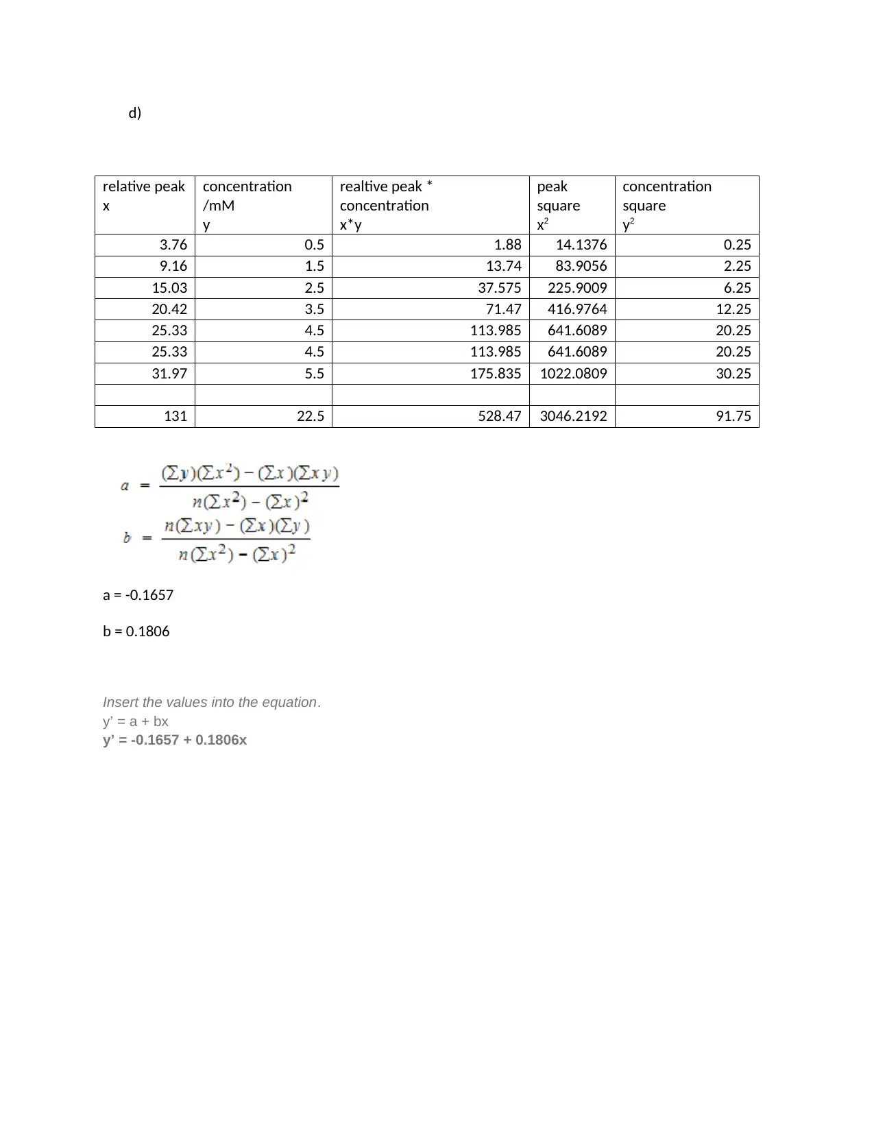
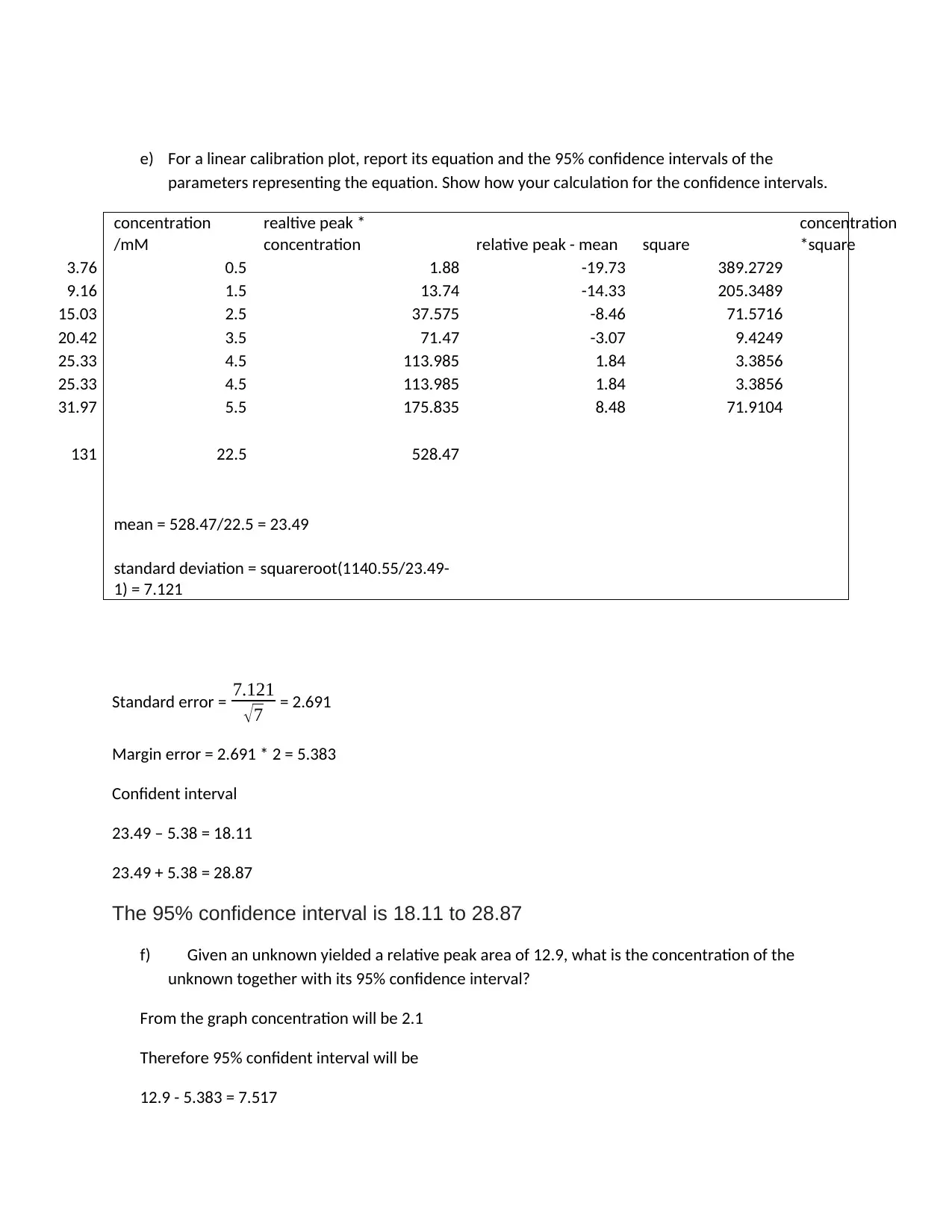
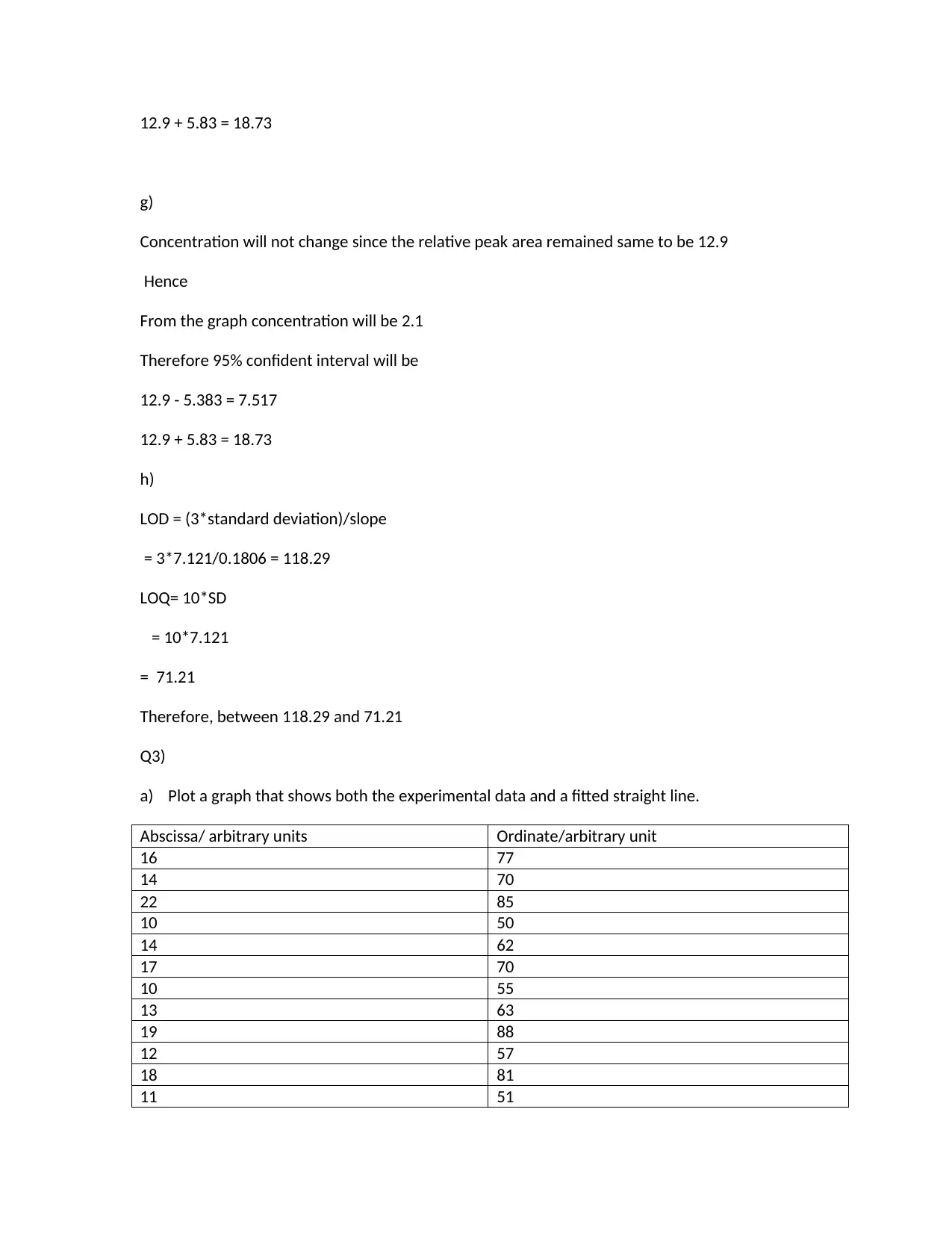
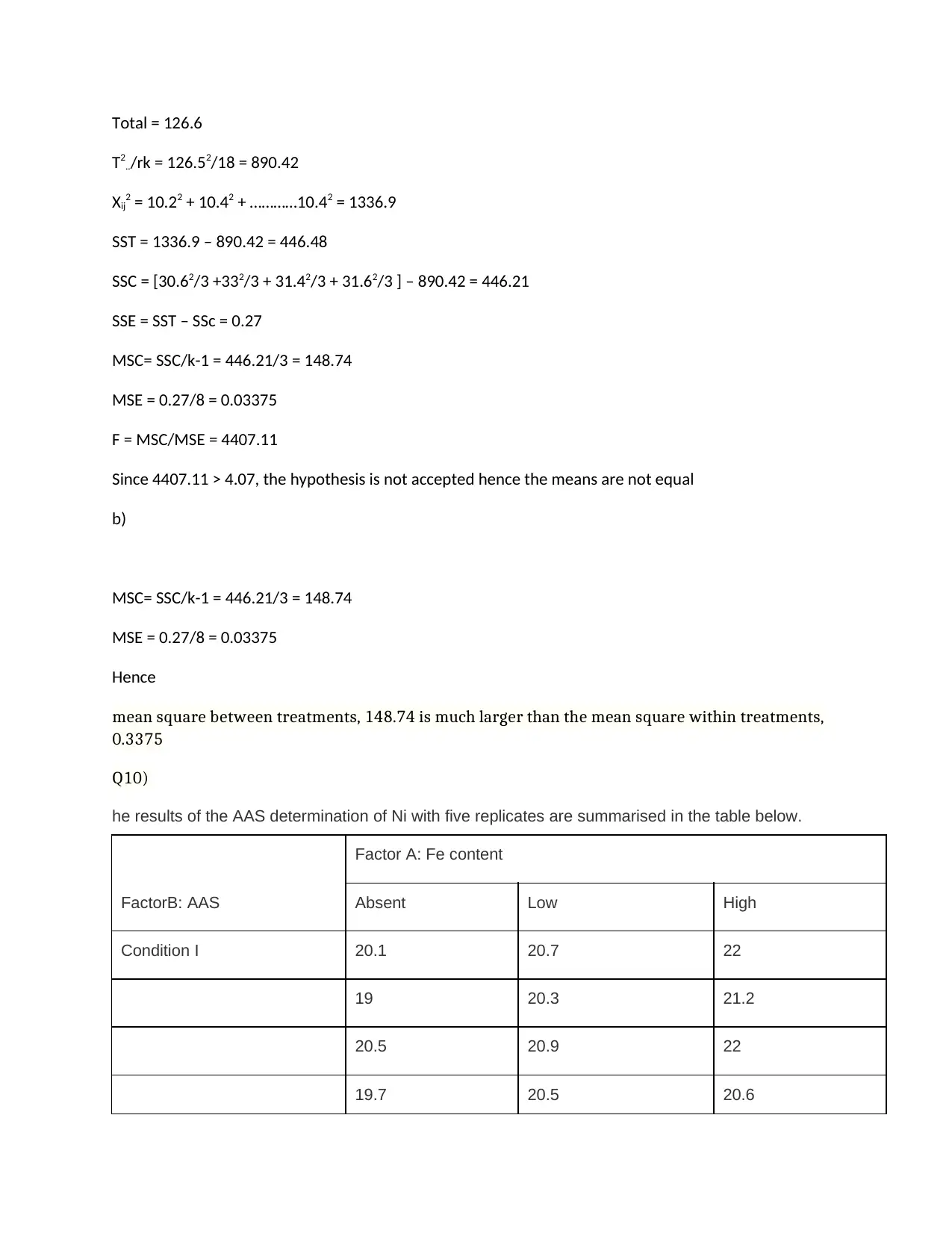
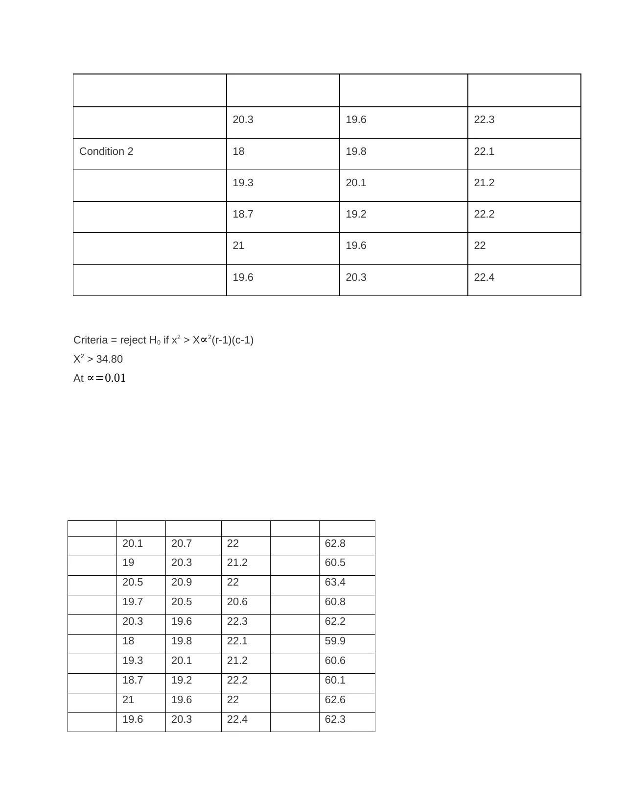
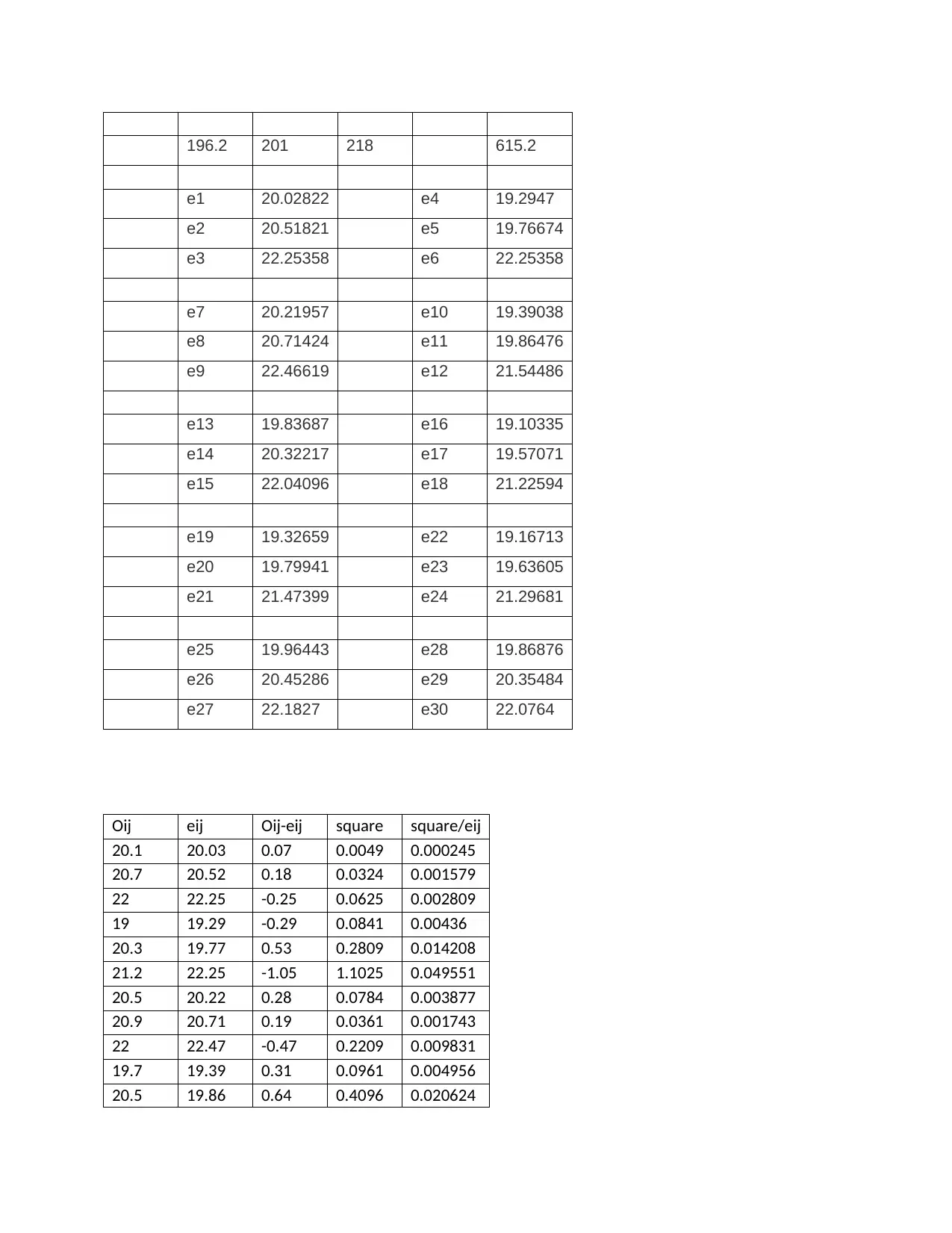
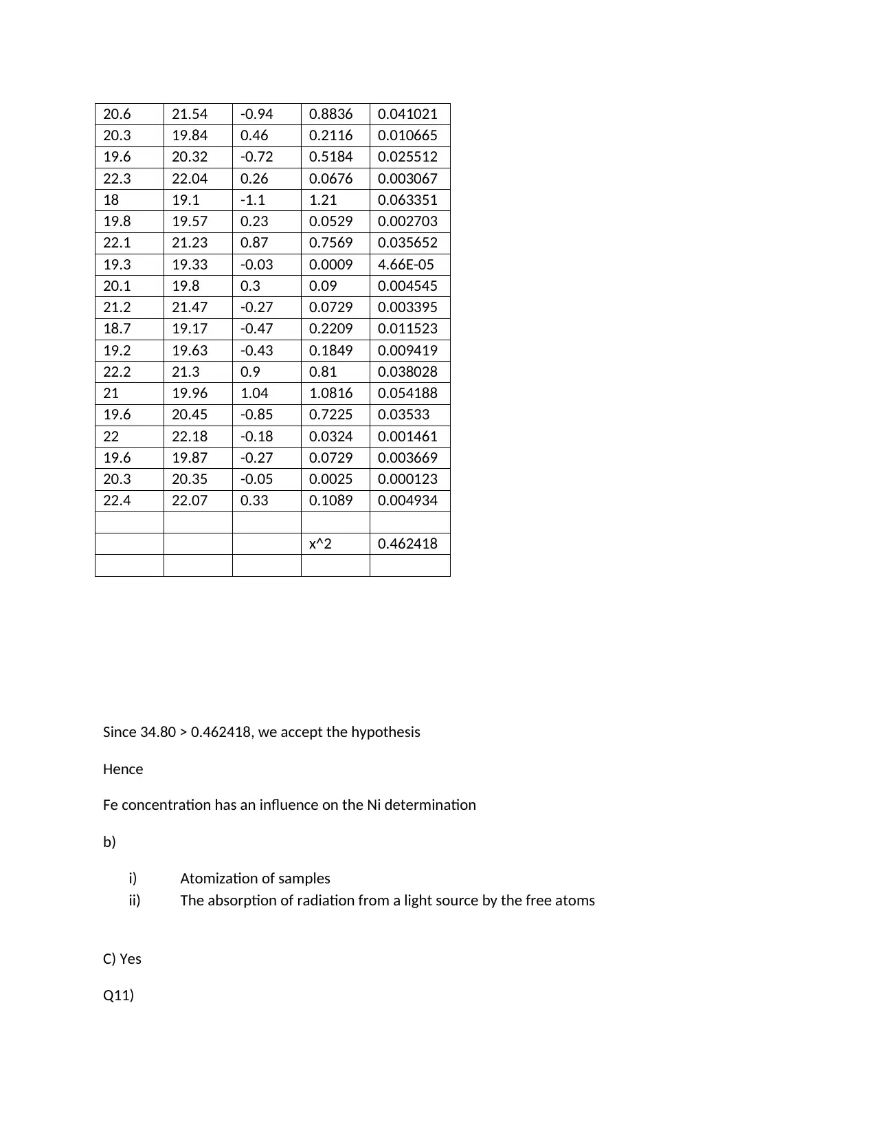
This document presents a comprehensive solution to a chemistry assignment, addressing various analytical chemistry concepts. The solution includes detailed calculations and explanations for calibration plots, statistical analysis, and the determination of confidence intervals. Furthermore, the document explores the application of statistical methods, such as ANOVA, to assess data and determine the significance of results. Additionally, the solution covers the Cumulative Sum (CUSUM) method for process control and provides an analysis of Atomic Absorption Spectroscopy (AAS) data, including the influence of factors on Ni determination. The assignment encompasses a wide range of topics, providing a thorough understanding of analytical techniques and statistical principles.

Q2)
a) Why must the concentration “0.500 mM” be reported to 3 decimal places in the above table?
This is because data should not be reported beyond the accuracy
of its determination. The 3 decimal places will be determined by
the confidence interval around the standard curve.
b) Why does the measurement parameter in the above table have no units?
The parameters are taken in comparison to each other which means the units will cancel out
c) Construct a graph that shows both the experimental data and a linear calibration plot.
Concentration /mM Relative peak area
0.500 3.76
1.50 9.16
2.50 15.03
3.50 20.42
4.50 25.33
5.50 31.93
0 5 10 15 20 25 30 35
0
1
2
3
4
5
6
f(x) = 0.180608717612039 x − 0.165677429596737
R² = 0.998381086864376
relative peak
concentration/mM

d)
relative peak
x
concentration
/mM
y
realtive peak *
concentration
x*y
peak
square
x2
concentration
square
y2
3.76 0.5 1.88 14.1376 0.25
9.16 1.5 13.74 83.9056 2.25
15.03 2.5 37.575 225.9009 6.25
20.42 3.5 71.47 416.9764 12.25
25.33 4.5 113.985 641.6089 20.25
25.33 4.5 113.985 641.6089 20.25
31.97 5.5 175.835 1022.0809 30.25
131 22.5 528.47 3046.2192 91.75
a = -0.1657
b = 0.1806
Insert the values into the equation.
y’ = a + bx
y’ = -0.1657 + 0.1806x

e) For a linear calibration plot, report its equation and the 95% confidence intervals of the
parameters representing the equation. Show how your calculation for the confidence intervals.
concentration
/mM
realtive peak *
concentration relative peak - mean square
concentration
*square
3.76 0.5 1.88 -19.73 389.2729
9.16 1.5 13.74 -14.33 205.3489
15.03 2.5 37.575 -8.46 71.5716
20.42 3.5 71.47 -3.07 9.4249
25.33 4.5 113.985 1.84 3.3856
25.33 4.5 113.985 1.84 3.3856
31.97 5.5 175.835 8.48 71.9104
131 22.5 528.47
mean = 528.47/22.5 = 23.49
standard deviation = squareroot(1140.55/23.49-
1) = 7.121
Standard error = 7.121
√7 = 2.691
Margin error = 2.691 * 2 = 5.383
Confident interval
23.49 – 5.38 = 18.11
23.49 + 5.38 = 28.87
The 95% confidence interval is 18.11 to 28.87
f) Given an unknown yielded a relative peak area of 12.9, what is the concentration of the
unknown together with its 95% confidence interval?
From the graph concentration will be 2.1
Therefore 95% confident interval will be
12.9 - 5.383 = 7.517

12.9 + 5.83 = 18.73
g)
Concentration will not change since the relative peak area remained same to be 12.9
Hence
From the graph concentration will be 2.1
Therefore 95% confident interval will be
12.9 - 5.383 = 7.517
12.9 + 5.83 = 18.73
h)
LOD = (3*standard deviation)/slope
= 3*7.121/0.1806 = 118.29
LOQ= 10*SD
= 10*7.121
= 71.21
Therefore, between 118.29 and 71.21
Q3)
a) Plot a graph that shows both the experimental data and a fitted straight line.
Abscissa/ arbitrary units Ordinate/arbitrary unit
16 77
14 70
22 85
10 50
14 62
17 70
10 55
13 63
19 88
12 57
18 81
11 51

8 10 12 14 16 18 20 22 24
0
10
20
30
40
50
60
70
80
90
100
f(x) = 3.26890756302521 x + 19.4726890756303
R² = 0.889117714996675
Y-Values
Abscissa/arbitrary unit
ordinate /arbitrary unit
b)
abscissa/arbitrary unit
(X)
ordinate/arbitrary
unit (Y)
X*Y square X square Y
16 77 1232 256 5929
14 70 980 196 4900
22 85 1870 484 7225
10 50 500 100 2500
14 62 868 196 3844
17 70 1190 289 4900
10 55 550 100 3025
13 63 819 169 3969
19 88 1672 361 7744
12 57 684 144 3249
18 81 1458 324 6561
11 51 561 121 2601
176 809 12384 2740 56447

a = 19.47
b = 3.27
Insert the values into the equation.
y’ = a + bx
y’ = 19.47 – 3.27x
c)
abscissa/
arbitrary unit (X)
ordinate/
arbitrary unit (Y)
X*Y Y-mean square x*square
16 77 1232 6.64 44.0896 705.4336
14 70 980 -0.36 0.1296 1.8144
22 85 1870 14.64 214.3296 4715.2512
10 50 500 -20.36 414.5296 4145.296
14 62 868 -8.36 69.8896 978.4544
17 70 1190 -0.36 0.1296 2.2032
10 55 550 -15.36 235.9296 2359.296
13 63 819 -7.36 54.1696 704.2048
19 88 1672 17.64 311.1696 5912.2224
12 57 684 -13.36 178.4896 2141.8752
18 81 1458 10.64 113.2096 2037.7728
11 51 561 -19.36 374.8096 4122.9056
176 809 12384 27826.7296
mean =
12384/176 =
70.36
standard deviation =
squareroot(27826.73/176-1) = 12.61

Standard error = 12.61
√12 = 3.64
Margin error = 3.64 * 2 = 7.28
Confident interval
70.36 – 7.28 = 63.08
70.36 + 5.38 = 77.64
The 95% confidence interval is 63.08 to 77.64
d)
8 10 12 14 16 18 20 22 24
-40
-20
0
20
40
60
80
100
ordinate/arbitrary unit (Y)
#VALUE!
e)

8 10 12 14 16 18 20 22 24
-40
-20
0
20
40
60
80
100
ordinate/arbitrary unit (Y)
#VALUE!
(i) Weighted plots are performed in calculating the various indices that affects the resulting
index value, as compared with the unweighted plots.
(ii) Where visual field damage is only peripheral, the unweighted index will be larger than the
corresponding weighted one.
Q9)
Criteria: reject F>F ∝[k-1,k(r-1)]
K = 4, r =3
F0.05(3, 8) = 4.07
Reject H0 if F> 4.07
Calculation
T1. = 30.6
T2. = 33
T3. = 31.4
T4. = 31.6

Total = 126.6
T2../rk = 126.52/18 = 890.42
Xij2 = 10.22 + 10.42 + …………10.42 = 1336.9
SST = 1336.9 – 890.42 = 446.48
SSC = [30.62/3 +332/3 + 31.42/3 + 31.62/3 ] – 890.42 = 446.21
SSE = SST – SSc = 0.27
MSC= SSC/k-1 = 446.21/3 = 148.74
MSE = 0.27/8 = 0.03375
F = MSC/MSE = 4407.11
Since 4407.11 > 4.07, the hypothesis is not accepted hence the means are not equal
b)
MSC= SSC/k-1 = 446.21/3 = 148.74
MSE = 0.27/8 = 0.03375
Hence
mean square between treatments, 148.74 is much larger than the mean square within treatments,
0.3375
Q10)
he results of the AAS determination of Ni with five replicates are summarised in the table below.
FactorB: AAS
Factor A: Fe content
Absent Low High
Condition I 20.1 20.7 22
19 20.3 21.2
20.5 20.9 22
19.7 20.5 20.6

20.3 19.6 22.3
Condition 2 18 19.8 22.1
19.3 20.1 21.2
18.7 19.2 22.2
21 19.6 22
19.6 20.3 22.4
Criteria = reject H0 if x2 > X∝2(r-1)(c-1)
X2 > 34.80
At ∝=0.01
20.1 20.7 22 62.8
19 20.3 21.2 60.5
20.5 20.9 22 63.4
19.7 20.5 20.6 60.8
20.3 19.6 22.3 62.2
18 19.8 22.1 59.9
19.3 20.1 21.2 60.6
18.7 19.2 22.2 60.1
21 19.6 22 62.6
19.6 20.3 22.4 62.3

196.2 201 218 615.2
e1 20.02822 e4 19.2947
e2 20.51821 e5 19.76674
e3 22.25358 e6 22.25358
e7 20.21957 e10 19.39038
e8 20.71424 e11 19.86476
e9 22.46619 e12 21.54486
e13 19.83687 e16 19.10335
e14 20.32217 e17 19.57071
e15 22.04096 e18 21.22594
e19 19.32659 e22 19.16713
e20 19.79941 e23 19.63605
e21 21.47399 e24 21.29681
e25 19.96443 e28 19.86876
e26 20.45286 e29 20.35484
e27 22.1827 e30 22.0764
Oij eij Oij-eij square square/eij
20.1 20.03 0.07 0.0049 0.000245
20.7 20.52 0.18 0.0324 0.001579
22 22.25 -0.25 0.0625 0.002809
19 19.29 -0.29 0.0841 0.00436
20.3 19.77 0.53 0.2809 0.014208
21.2 22.25 -1.05 1.1025 0.049551
20.5 20.22 0.28 0.0784 0.003877
20.9 20.71 0.19 0.0361 0.001743
22 22.47 -0.47 0.2209 0.009831
19.7 19.39 0.31 0.0961 0.004956
20.5 19.86 0.64 0.4096 0.020624

20.6 21.54 -0.94 0.8836 0.041021
20.3 19.84 0.46 0.2116 0.010665
19.6 20.32 -0.72 0.5184 0.025512
22.3 22.04 0.26 0.0676 0.003067
18 19.1 -1.1 1.21 0.063351
19.8 19.57 0.23 0.0529 0.002703
22.1 21.23 0.87 0.7569 0.035652
19.3 19.33 -0.03 0.0009 4.66E-05
20.1 19.8 0.3 0.09 0.004545
21.2 21.47 -0.27 0.0729 0.003395
18.7 19.17 -0.47 0.2209 0.011523
19.2 19.63 -0.43 0.1849 0.009419
22.2 21.3 0.9 0.81 0.038028
21 19.96 1.04 1.0816 0.054188
19.6 20.45 -0.85 0.7225 0.03533
22 22.18 -0.18 0.0324 0.001461
19.6 19.87 -0.27 0.0729 0.003669
20.3 20.35 -0.05 0.0025 0.000123
22.4 22.07 0.33 0.1089 0.004934
x^2 0.462418
Since 34.80 > 0.462418, we accept the hypothesis
Hence
Fe concentration has an influence on the Ni determination
b)
i) Atomization of samples
ii) The absorption of radiation from a light source by the free atoms
C) Yes
Q11)