Civil Engineering Project: Hydrological Analysis of Catchment Areas

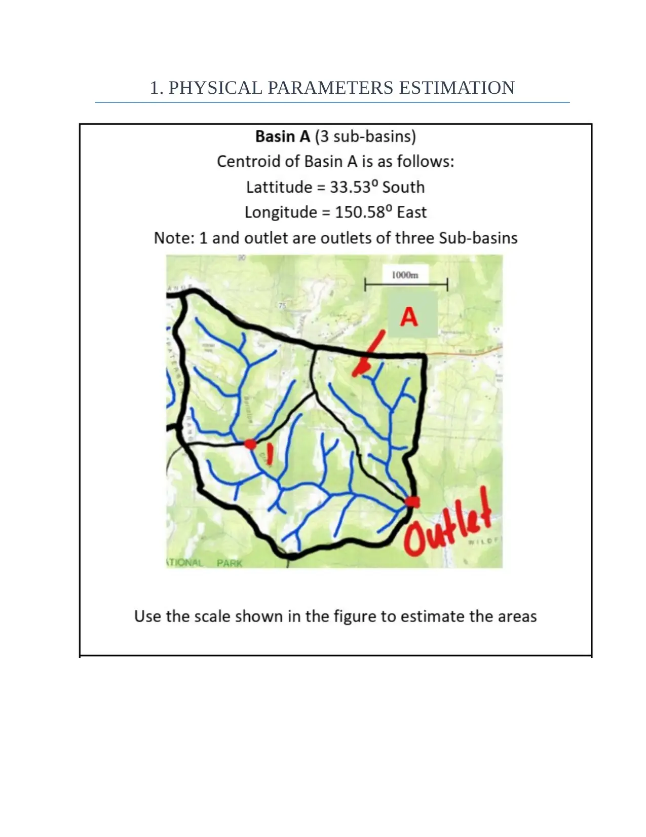
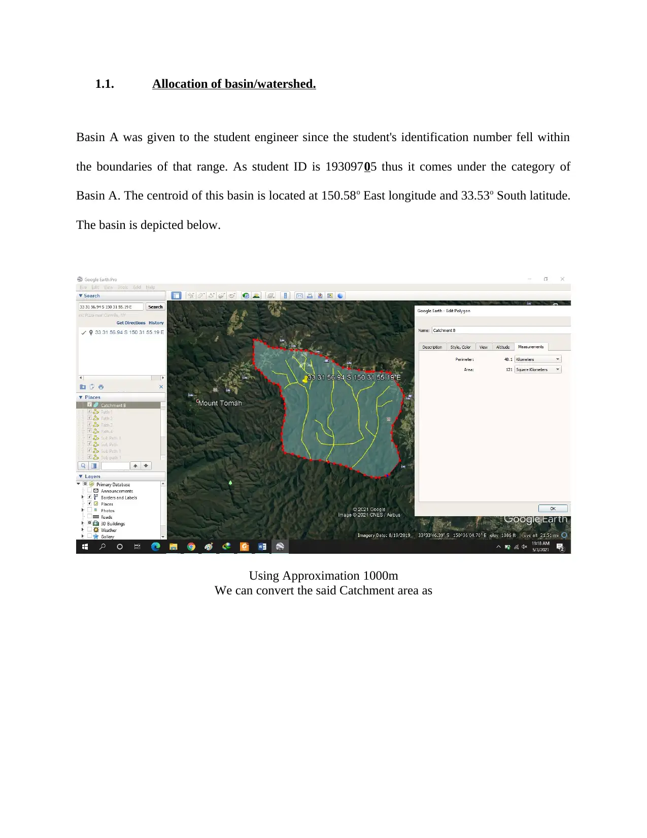
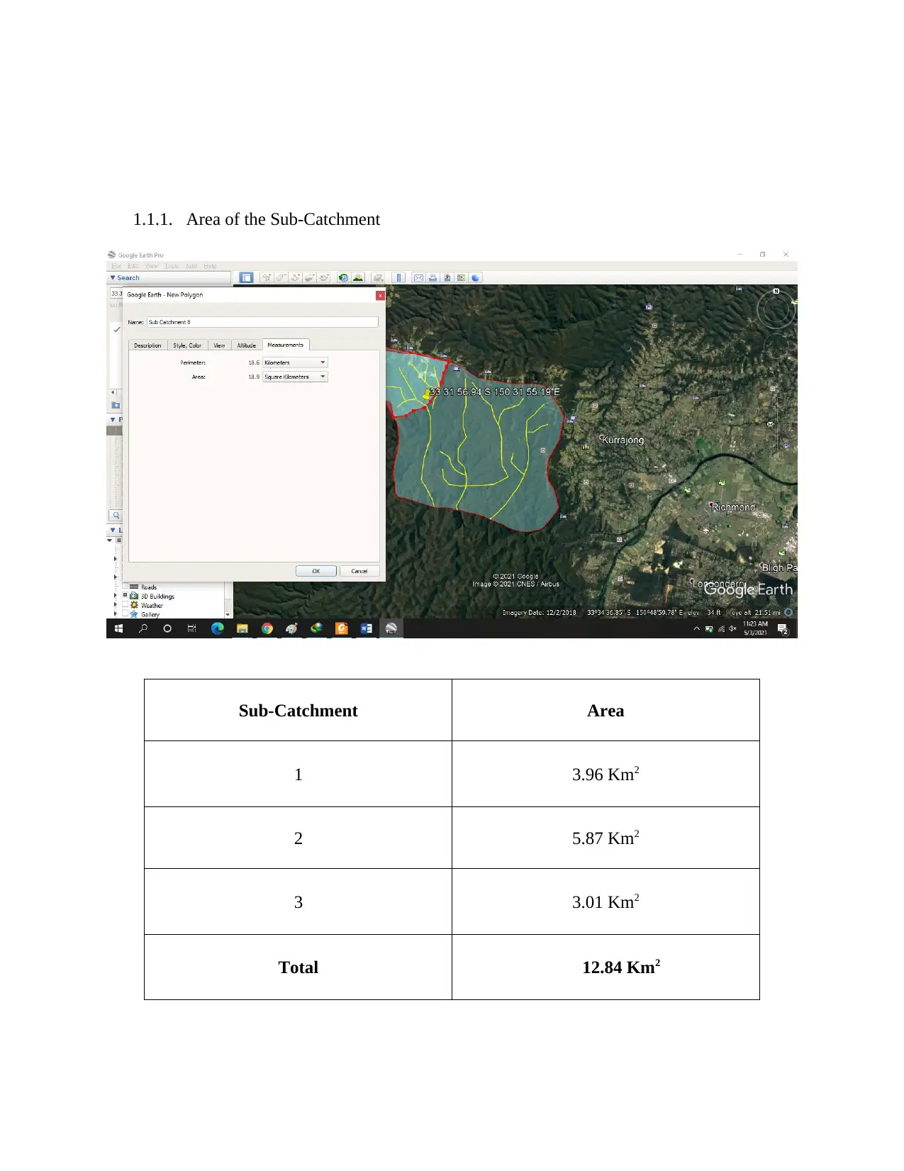
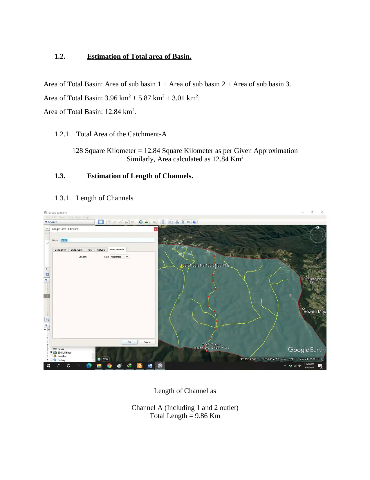
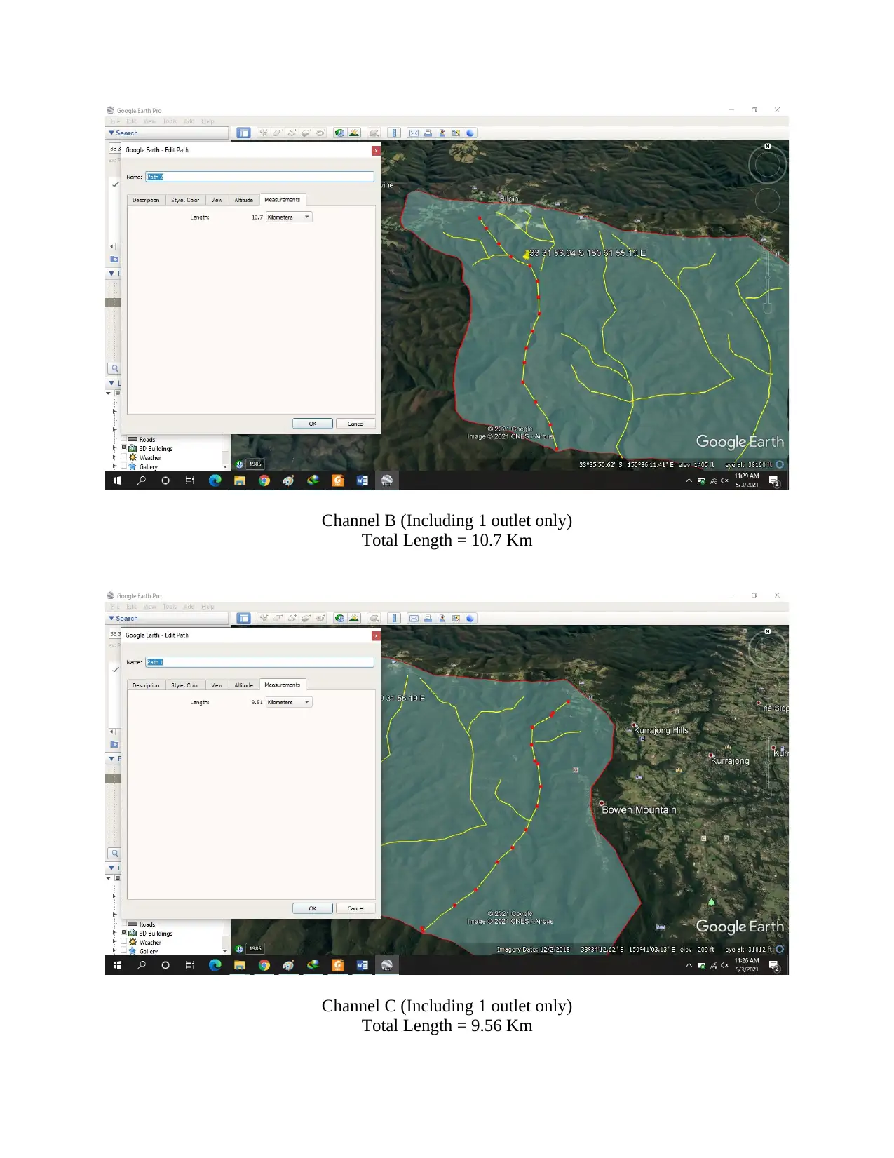
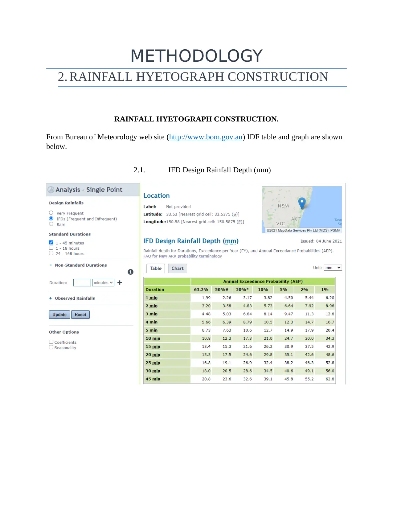
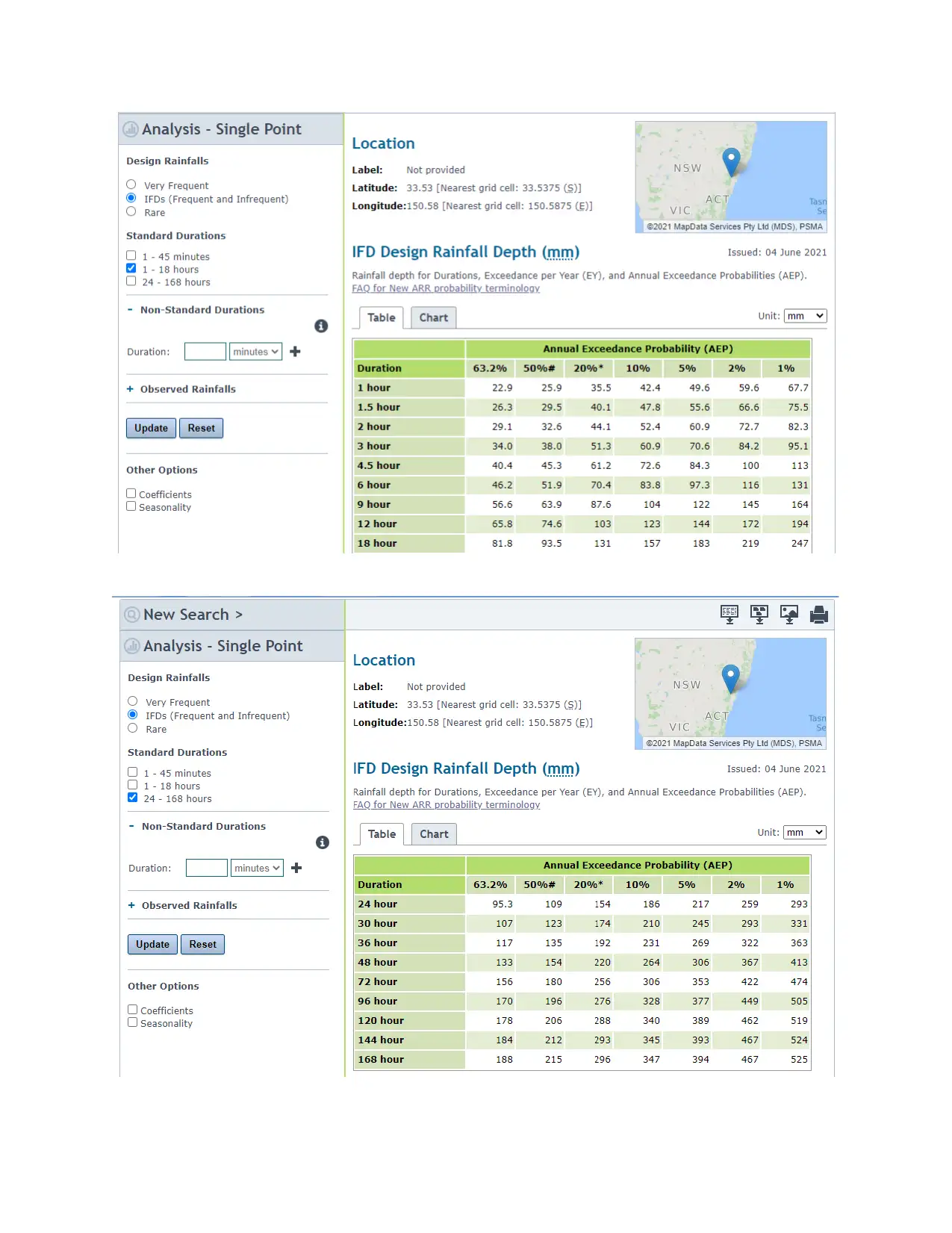
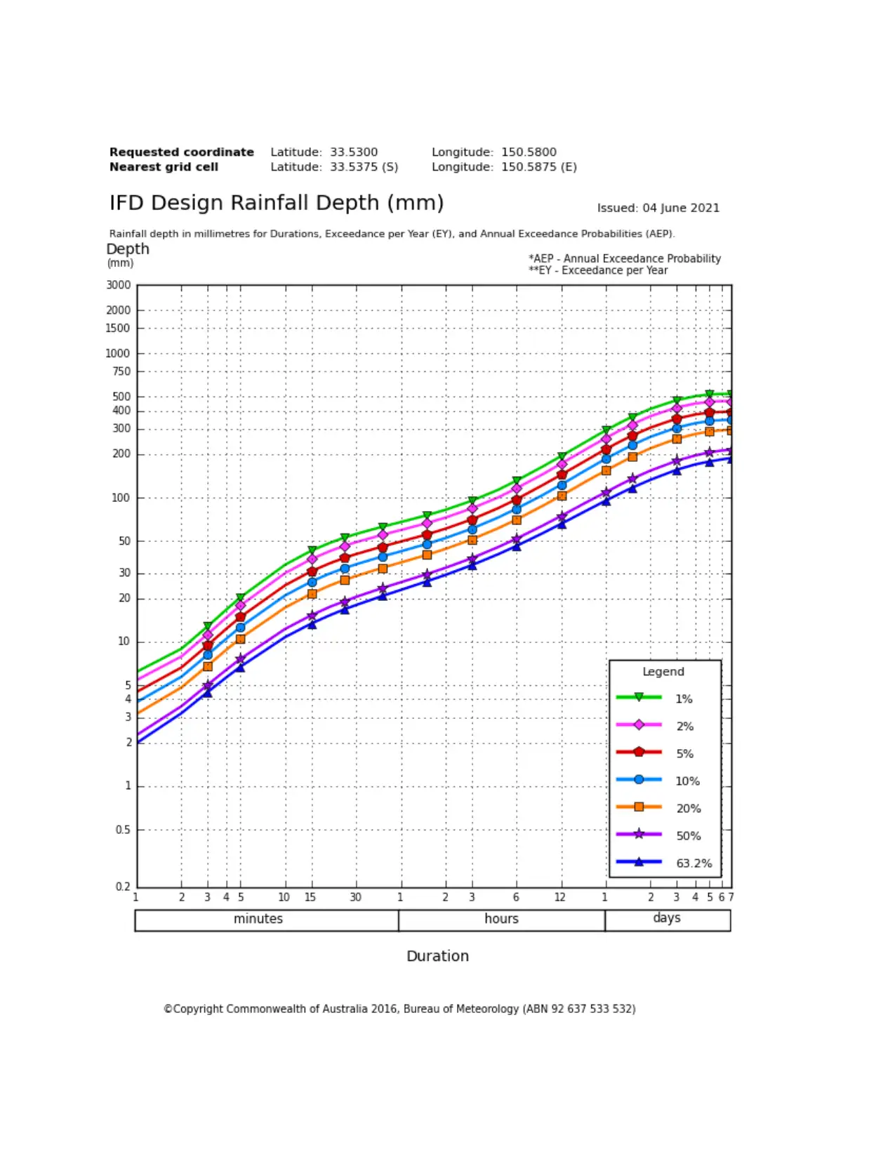
This project focuses on evaluating variations in catchment response behavior in pre-developed and post-developed settings within a specific region. It involves estimating physical parameters, constructing rainfall hyetographs, and generating storm hydrographs. The methodology includes detailed steps for rainfall analysis, excess hyetograph construction, desired duration unit hydrograph construction, and network diagram creation. The student engineer must apply critical thinking and engineering judgments to address potential challenges and create a functional design. The project utilizes learning models and computational simulations, including verification using HEC-HMS, to analyze the floodplain of the catchment areas. The analysis covers various aspects of hydrology, including rainfall, runoff, and the impact of urban development, with the aim of providing solutions to mitigate potential risks and improve water management. The project also involves obtaining and processing temporal rainfall data from the ARR website and applying relevant formulas for accurate hydrological analysis. The student must consider the effect of various parameters such as area, length, and time, for complete project analysis.

Contents
SCOPE........................................................................................................................................................2
INTRODUCTION.......................................................................................................................................3
STEP 1: PHYSICAL PARAMETERS ESTIMATION...............................................................................5
METHODLOGY
STEP 2: RAINFALL HYETOGRAPH CONSTRUCTION........................................................................9
STEP 4: DESIRED DURATION UNIT HYETOGRAPH CONSTRUCTION.........................................18
STEP 5: STORM HYETOGRAPH COMPUTATION..............................................................................24
STEP 6: NETWORK DIAGRAM CONSTRUCTION..............................................................................28
STEP 7: CONSTRUCTION OF POST DEVELOPMENT HYDROGRAPH...........................................34
STEP 8: VARIFICATION BY HEC HMS................................................................................................42
CONCLUSION.........................................................................................................................................52

SCOPE
This research aims to evaluate and evaluate variations in catchment response behavior in pre-
developed and post-developed settings within a specific region and to propose solutions that can
address possible difficulties along the route.
The physical parameters for the clock and the generation of the respective rainfall patterns and
storm hydrographs will include an evaluation of different parameters and the application of
various techniques to fulfil the tasks indicated in the project brief to achieve the correct definitive
results for the clock assigned.
In order to overcome problems and create a functional and safe design in compliance with the
directives of the Council, critical thinking, analytical skills and Engineering judgments will have
to be implemented at various stages of the project design and analysis by the student engineer.
The project gives the student engineer the capacity to examine and plan the floodplain of the
catchment areas during the pre-development and post-development process. Furthermore, the
student engineer could offer a response to challenges that could develop at any time in the
project.
For the development of the project, several learning models and computational simulation should
be employed and a real-life problem that needs to be solved should be associated and worked on.
INTRODUCTION
Hydrology is important to civil and environmental engineers, hydro geologists, and earth
scientists, and it plays an important part in water management, droughts, and floods, as well as
the techniques for dealing with them. Issues relating to urban storm water and runoff, water

safety, and watershed conservation have prompted comprehensive and in-depth studies and
measures to be implemented in order to protect water balance and support productive production
while minimizing potential risks. Multiple storm events (such as hurricanes, cyclones, torrential
rains, and so on) have triggered major urban disasters in recent years, particularly in coastal areas
where economic growth has been rapid, and potential responses to these problematic events
(Bedient, Huber, and Vieux) must be investigated and addressed.
The total amount of precipitation (also known as rainfall) remains in the area where it fell and
contributes to the atmosphere through evaporation and transpiration (water vapors leaking
through plant tissue and leaves). Evapotranspiration is the term used to describe these two
mechanisms. Any water that reaches the surface causes infiltration. The permeability of the soil
and its ability to absorb and hold water have an impact on this mechanism. Percolation, the
process of replenishing groundwater sources, can begin after this stage. Pumping groundwater
for farm and urban water sources is possible (U.S. Geological Survey Agency, 2017).
When the surface is totally saturated or the surface has weak permeability properties, the
remainder of the precipitation goes overland or run-off. Run-off travels in a downward direction,
accumulating in isolated, local water sources before migrating to the main. This is the larger
body of water. Excess run-off is a parameter that needs to be addressed as cities grow (Loaiciga,
Valdes, Vogel, Garvey & Schwarz, 1996).
It is feasible to define regions where improvements in topography and construction can have a
significant impact on flood behaviour by being able to identify and consider floodways, and so
take a critical step toward recognising flood activity and developing viable flood control
techniques (Albert, Murtagh, Babister, McLuckie, 2017).

By increasing nutrient retention within the channel network and improving downstream water
quality, as well as raising channel roughness, effective approaches can be achieved, such as
mitigating channel erosion (protecting soil and reducing sediment supplies to downstream water
bodies), increasing nutrient retention within the channel network and improving downstream
water quality, and finally, decreasing floods in the lower catchment area.
Finally, with today's improved data on radar precipitation and moisture gauges, advanced
processing capacity, and improved hydraulic simulation tools, simulations covering wide regions
using diverse approaches may be easily analysed. This provides a lot of benefits, but it also
causes some uncertainty. This is because precipitation is the most important factor in calculating
runoff, and the improved spatial clarity provided by radars, when combined with computer
simulation, can aid in better understanding the total catchment response, as long as these
apparatuses and instruments are properly configured for the simulation to be performed. If proper
calibration can be ensured, efficient and accurate hydrological analysis for floodplain control
programmes and planning strategies can be implemented (Daly, Reichard, Hansell & Clark,
2016).

1. PHYSICAL PARAMETERS ESTIMATION

1.1. Allocation of basin/watershed.
Basin A was given to the student engineer since the student's identification number fell within
the boundaries of that range. As student ID is 19309705 thus it comes under the category of
Basin A. The centroid of this basin is located at 150.58o East longitude and 33.53o South latitude.
The basin is depicted below.
Using Approximation 1000m
We can convert the said Catchment area as

1.1.1. Area of the Sub-Catchment
Sub-Catchment Area
1 3.96 Km2
2 5.87 Km2
3 3.01 Km2
Total 12.84 Km2

1.2. Estimation of Total area of Basin.
Area of Total Basin: Area of sub basin 1 + Area of sub basin 2 + Area of sub basin 3.
Area of Total Basin: 3.96 km2 + 5.87 km2 + 3.01 km2.
Area of Total Basin: 12.84 km2.
1.2.1. Total Area of the Catchment-A
128 Square Kilometer = 12.84 Square Kilometer as per Given Approximation
Similarly, Area calculated as 12.84 Km2
1.3. Estimation of Length of Channels.
1.3.1. Length of Channels
Length of Channel as
Channel A (Including 1 and 2 outlet)
Total Length = 9.86 Km

Channel B (Including 1 outlet only)
Total Length = 10.7 Km
Channel C (Including 1 outlet only)
Total Length = 9.56 Km

METHODOLOGY
2. RAINFALL HYETOGRAPH CONSTRUCTION
RAINFALL HYETOGRAPH CONSTRUCTION.
From Bureau of Meteorology web site (http://www.bom.gov.au) IDF table and graph are shown
below.
2.1. IFD Design Rainfall Depth (mm)

2.2. IFD
Design Rainfall Intensity (mm/h)

2.3. Data From ARR Website
Temporal Data was downloaded from ARR website (https://data.arr-software.org/).

Temporal Data was downloaded from ARR website (https://data.arr-software.org/).

Temporal Rainfall Pattern data was obtained from website. As a consequence of design rainfall
for AEP=9 percent it was found to be rare, only infrequent / intermediate 24-hour rainfall data
from the derived file is considered. These are as follows (the selected objects shown in the
diagram below):
Burst Duration
(min) Burst Loading Original Burst
Depth (mm) AEP Window AEP (source) (%)
10 1 18.2 intermediate 9.0626
20 1 30 intermediate 9.1523
20 3 37.89 intermediate 9.2486
25 1 40.4 intermediate 9.2365
25 2 32.5 intermediate 9.8770
25 3 33 intermediate 9.7451
30 3 27.79 intermediate 9.9771
45 2 33.11 intermediate 9.269
120 2 87 intermediate 9.2057
180 1 74.31 intermediate 9.5251
270 1 88.75 intermediate 9.3369
270 2 56.11 intermediate 9.0568
360 1 56.4 intermediate 9.5924
540 2 99.82 intermediate 9.9007
720 2 129.14 intermediate 9.2865
1080 3 136.52 intermediate 9.9109
1080 3 102.91 intermediate 9.9149
1440 1 116.19 intermediate 9.4002
2160 1 156.54 intermediate 9.5394
4320 3 183.64 intermediate 9.0424
7200 2 219.11 intermediate 9.4659
10080 2 310.51 intermediate 9.8241
Relationship used here is
AEP = 1−e( −1
ARI )
AEP = 1−e(−1
10 ) = 1-0.90483 =0.095*100 = 9.5%
As per above data we can calculate the depth as
Considering duration of rain is 6 hours
Then

As per AEP = 9% Duration 9 hours the Depth will be
50.8 mm
(As Per Latest Method of Calculation)
Temporal Data was downloaded from ARR website (https://data.arr-software.org/).
3. Gross Rainfall Hydrograph
Single average incremental rainfall distribution for every 15-minute increment is used for all other
because simultaneous analysis is not required.
Rainfall % for first 15 mins= ( 3.88+5.84+9.30+10.7+12.9+21.3+26.5+ 28.4+31.36 )
9
Rainfall %for first 15 mins=16.68 %
Same formula is used to calculate other sample calculations.
Rainfall Depth for first 15 mins=73.6 mm ×16.68 %=12.27 mm
Event ID Duration Time Step Region AEP 15
4669 180 15 East Coast (South) frequent 12.46
4670 180 15 East Coast (South) frequent 12.97
4673 180 15 East Coast (South) frequent 11.6
4674 180 15 East Coast (South) frequent 9.67
4675 180 15 East Coast (South) frequent 9.64
4676 180 15 East Coast (South) frequent 27.25
4677 180 15 East Coast (South) frequent 4.2
4679 180 15 East Coast (South) frequent 5.05
4681 180 15 East Coast (South) frequent 15.04
4627 180 15 East Coast (South) intermediate 7.25
Average rainfall Depth (mm) 72.9 Average ARR increment 11.51
Rainfall depth (mm) 6.86
Rainfall intensity =12.27 x ( 60
15 )=49.08 mm

Time ARR (%) Depth (mm) Rainfall intensity (mm/hr)
0-15 9.07 7.54 30.17
15-30 7.24 6.02 24.08
30-45 9.16 7.62 30.47
45-60 10.61 8.83 35.31
60-75 6.80 5.66 22.63
75-90 7.96 6.62 26.50
90-105 8.91 7.41 29.64
105-120 7.67 6.38 25.51
120-135 7.62 6.34 25.34
135-150 8.36 6.96 27.83
150-165 8.03 6.68 26.72
165-180 8.60 7.15 28.61
0-15 15-30 30-45 45-60 60-75 75-90 90-105 105-
120 120-
135 135-
150 150-
165 165-
180
0.00
5.00
10.00
15.00
20.00
25.00
30.00
35.00
40.00
Gross Rainfall Hyetograph.
Duration
Intensity (mm/hr)

4. RAINFALL EXCESS
HYETOGRAPH CONSTRUCTION.

4.1. ARF Parameters

4.2. Median Pre-burst Depths and Ratios

4.3. Interim Climate Change Factors

Following important data has been extracted:
- Total rainfall depth = 73.6 mm
- Initial Loss = 22 mm
- Continuing Loss = 1.8 mm/hr.
Continuing Loss = 0.45 mm/ 15 min.
First interval excess rain: 30.26 – 22 = 8.26 mm
Time to reach initial loss: (15/30.26) x 23 =11.40 min.
Continuous loss: (15-11.40) x 0.45 mm/ 15 min. = 0.108 mm.
Net Rainfall: 7.14 mm - 0.108 mm. = 7.032 mm.
Loss: 7.54 mm - 7.032 mm. = 0.418 mm.
All other losses will be: 0.45 mm.
Time ARR
(%)
Depth
(mm)
Rainfall
intensity
(mm/hr)
Gross Rainfall
depth (mm)
Cumulative
Rainfall depth
Loss Net
Rainfall
(mm)
0-15 9.07 7.54 30.17 30.17 30.17 0.489 7.054
15-30 7.24 6.02 24.08 24.08 54.25 0.375 5.645
30-45 9.16 7.62 30.47 30.47 84.72 0.375 7.242
45-60 10.61 8.83 35.31 35.31 120.03 0.375 8.453
60-75 6.80 5.66 22.63 22.63 142.66 0.375 5.283
75-90 7.96 6.62 26.50 26.50 169.16 0.375 6.249
90-105 8.91 7.41 29.64 29.64 198.79 0.375 7.035
105-120 7.67 6.38 25.51 25.51 224.30 0.375 6.002
120-135 7.62 6.34 25.34 25.34 249.65 0.375 5.961
135-150 8.36 6.96 27.83 27.83 277.48 0.375 6.582
150-165 8.03 6.68 26.72 26.72 304.19 0.375 6.304
165-180 8.60 7.15 28.61 28.61 332.80 0.375 6.777
Green region shows losses and Blue region is depth of excess rain fall.

0-15 15-30 30-45 45-60 60-75 75-90 90-105 105-
120 120-
135 135-
150 150-
165 165-
180
0.000
1.000
2.000
3.000
4.000
5.000
6.000
7.000
8.000
9.000
10.000
Gross Rainfall Hyetograph (pre dev)
duration
NET DETH (mm)
5. DESIRED DURATION UNIT
HYETOGRAPH CONSTRUCTION.

For 5-minute hydrograph construction for provided sub basins, sub basin areas need to be scaled
with area of provided data of 5-minute hydrograph. Provided data is as follows,
Time (min) 5 min UH
Q (m3/sec)
0 0
5 1.02
10 2.34
15 4.26
20 5.172
25 4.38
30 3.54
35 2.58
40 1.908
45 1.38
50 1.02
55 0.78
60 0.54
65 0.42
70 0.3
75 0.24
80 0.12
85 0
Area 600 hectares
Area of sub basin 1: 3.96 km2. = 396 hectares.
Area of sub basin 2: 5.87 km2. = 587 hectares.
Area of sub basin 3: 3.01 km2. = 301 hectares.
5 min discharge for sub basin 1 will be: 0.85 x (396/600) = 0.561 m3/s.
All additional calculations are carried out in the same manner.
Time (min) 5 min UH Scaling of Sub Basins
Q (m3/sec) Q1 (m3/sec) Q2 (m3/sec) Q3 (m3/sec)
0 0 0.000 0.000 0.000
5 0.85 1.419 0.790 0.989
10 1.95 3.255 1.812 2.270
15 3.55 5.926 3.299 4.132
20 4.31 7.195 4.005 5.017

25 3.65 6.093 3.392 4.249
30 2.95 4.925 2.742 3.434
35 2.15 3.589 1.998 2.503
40 1.59 2.654 1.478 1.851
45 1.15 1.920 1.069 1.339
50 0.85 1.419 0.790 0.989
55 0.65 1.085 0.604 0.757
60 0.45 0.751 0.418 0.524
65 0.35 0.584 0.325 0.407
70 0.25 0.417 0.232 0.291
75 0.2 0.334 0.186 0.233
80 0.1 0.167 0.093 0.116
85 0 0.000 0.000 0.000
Area 750 hectares 41.733 23.233 29.100
Unit Hydrograph of Sub basin 1.
0 10 20 30 40 50 60 70 80 90
0.000
1.000
2.000
3.000
4.000
5.000
6.000
7.000
8.000
5 min UH of sub basin 1
time (min)
discharge (m3/sec)
Unit Hydrograph of Sub basin 2.

0 10 20 30 40 50 60 70 80 90
0.000
0.500
1.000
1.500
2.000
2.500
3.000
3.500
4.000
4.500
5 min UH of sub basin 2
time (min)
discharge (m3/sec)
Unit Hydrograph of Sub basin 3.
0 10 20 30 40 50 60 70 80 90
0.000
1.000
2.000
3.000
4.000
5.000
6.000
5 min UH of sub basin 2
time (min)
discharge (m3/sec)
Unit Hydrograph of all 3 Sub-basins

0 10 20 30 40 50 60 70 80 90
0.000
1.000
2.000
3.000
4.000
5.000
6.000
7.000
8.000
5 min UH of three sub basins
time (min)
discharge (m3/sec)
15 min UH data sub basin 1.
Time (min) Q (m/sec) Q1 (m3/sec) 5 min lag (1) 5 min lag (2) Total 15
min H=
4mm
Total 15
min H=
1mm
0 0 0.000 0.000 0.000
5 0.85 1.419 0.000 1.419 0.355
10 1.95 3.255 1.419 0.000 4.674 1.169
15 3.55 5.926 3.255 1.419 10.600 2.650
20 4.31 7.195 5.926 3.255 16.376 4.094
25 3.65 6.093 7.195 5.926 19.214 4.804
30 2.95 4.925 6.093 7.195 18.212 4.553
35 2.15 3.589 4.925 6.093 14.607 3.652
40 1.59 2.654 3.589 4.925 11.168 2.792
45 1.15 1.920 2.654 3.589 8.163 2.041
50 0.85 1.419 1.920 2.654 5.993 1.498
55 0.65 1.085 1.419 1.920 4.424 1.106
60 0.45 0.751 1.085 1.419 3.255 0.814
65 0.35 0.584 0.751 1.085 2.421 0.605
70 0.25 0.417 0.584 0.751 1.753 0.438
75 0.2 0.334 0.417 0.584 1.335 0.334
80 0.1 0.167 0.334 0.417 0.918 0.230
85 0 0.000 0.167 0.334 0.501 0.125
90 0.000 0.167 0.167 0.042
95 0.000 0.000 0.000

0 10 20 30 40 50 60 70 80 90 100
0.000
5.000
10.000
15.000
20.000
25.000
15 min hydrgraph sub basin 1
Q1 (m3/sec) 5 min lag (1)
5 min lag (2) Total 15 min H= 4mm
time
discharge
5.1. Removal of Base Flow
5.2. Calculation of unit hydrograph at given 9-hour condition
5.3. Ordinate of unit hydrograph calculated at t = 09-hr:

QUH (09 hr) = (7.53m3/s) (1.065) = 8.630 m3/s

STEP 5: STORM HYETOGRAPH COMPUTATION.
For construction of storm hydro graph, 15 min hydro graph is required,
0 200 400 600 800 1000 1200 1400 1600
0.00
10.00
20.00
30.00
40.00
50.00
60.00
Storm Hydrograph basin 1
duration
discharge

Sub basin 2:
0 200 400 600 800 1000 1200 1400 1600
0.00
5.00
10.00
15.00
20.00
25.00
30.00
Storm Hydrograph basin 2
duration
discharge
Sub basin 3:

0 200 400 600 800 1000 1200 1400 1600
0.00
5.00
10.00
15.00
20.00
25.00
30.00
35.00
40.00
Storm Hydrograph basin 3
duration
discharge
From graphs, the peak discharge and time to reach peak is as follows,
Sub Basin 1 2 3
Peak discharge (Qp) m3/s 49.01 26.53 33.96
Peak time (Tp) min 467 467 467
Peak time (Tp) hours 7.82 7.82 7.82

6. NETWORK DIAGRAM
Basin A
Basin B
Outlet
Basin C

7. FOR UNIT HYDROGRAPH AND
STORM HYDROGRAPH, SEE THE
EXCEL SHET ATTACHED FOR
DETAILED CALCULATIONS
The same approach that was used to build pre-development storm hydrographs in tasks 3, 4, and
5 will be used to build post-development storm hydrographs in job 6. This assignment, on the
other hand, would take into consideration the expansion of certain of the watershed sub basins 2.
As a result, the student engineer decided to develop sub-catchment 3 as the precipitation excess
discharges straight to the watershed's departure point, eliminating the need to rebuild and/or re-
analyze the channel routing. Both the initial and ongoing losses will be reduced by 50%. The
following properties will be present in a 5-minute unit-hydrograph.
 Peak discharge will increase by 30%, while time to peak will be reduced by 15%.
 The time basis will be reduced by 25%.
Solution
Using Muskingum routing Method and Assuming x=0.2
And average channel velocity is 1.2m/sec
Time (Min) Discharge (m3/sec)
0 0
5 0.54
10 1.76
15 3.28
20 3.75
25 3.36
30 2.55
35 1.59
40 1.05

45 0.72
50 0.48
55 0.32
60 0.21
65 0.14
70 0.09
75 0.06
80 0.04
85 0.03
90 0.02
95 0.01
100 0
Calculation of basic parameters as
D = (K-Kx)*0.2+0.5Dt
D =(5-0.54)*0.2+0.5*3 = 4.89 + 1.5 = 6.39
Now Calculating C0
C0 = (0.5Dt-Kx)/D = (0.5*5-0.54*0.2)/6.39=0.07
Similarly, for C1
C1 = (0.54*0.2+0.5*5)/6.39=0.07=0.560
Similarly, for C2
C2 = (5-4.69*0.2-0.5*5)/6.39=0.07=0.38
Check if
C0 + C1 + C2 = 1
0.07 + 0.570 + 0.38 = 1.01 (Change the Largest Weight)
C1 = 0.55
Now using Routing equation
O2 = CoI2 + C1I1 + C2O1 = 0.07I2 + 0.55I1 + 0.38O2
Time (Min) Discharge (m3/sec) O (m3/sec)
0 0
5 0.54 0.46
10 1.76 1.50
15 3.28 2.79
20 3.75 3.19
25 3.36 2.86

30 2.55 2.45
35 1.59 1.88
40 1.05 1.28
45 0.72 0.98
0 5 10 15 20 25 30 35 40 45 50
0
0.5
1
1.5
2
2.5
3
3.5
4
0
0.54
1.76
3.28
3.75
3.36
2.55
1.59
1.05
0.72
Time (Min)
Discharge (m3/sec)

0 5 10 15 20 25 30 35 40 45
0
0.5
1
1.5
2
2.5
3
3.5
4
0
0.54
1.76
3.28
3.75
3.36
2.55
1.59
1.05
0.72
Time (Min)
Discharge (m3/sec)
Also include Muskingum HEC-HMS Files

8. COMPARISON OF PRE AND
POST DEVELOPEMENT GRAPH.
Various characteristics are quite obvious and straightforward while studying storm hydrographs
at the watershed's outlet point. The urbanization of a segment of the watershed has had
consequences and implications. The following are the hydrographs:
0 10 20 30 40 50 60 70 80 90 100
0.00
10.00
20.00
30.00
40.00
50.00
60.00
70.00
80.00
90.00
Pre and Post developed outflow storm
Outflow Basin Outflow Basin developed
duration
discharge
The impact of urbanization has clearly contributed to a change in the watershed's nature. The
length of the run-off for (time base), the peak discharge at the catchment area's outflow, and the
time it takes for the original peak discharge to occur have all improved in the catchment reaction.
The discharge is expected to rise by about 5%.
Discharge table values are shown below:
Discharge m3/s
Pre developed 76.36
Post developed 82.60

According to the Council Rules, while the catchment is being developed, the flow of water must
be managed and maintained below a certain amount in compliance with strict requirements. Any
amount of water released from a watershed outlet must be less than or equal to the highest
discharge generated before the catchment was constituted, according to the Guidelines.
The issue may be remedied by decreasing the impact of urbanization by recharging groundwater
and lowering peak discharge to allowable levels. Building a reservoir is another costlier solution
that is useless since it is not cost-effective.
Check Calculations in Excel Sheet Attached
9. VARIFICATION BY HEC HMS.

Attached HEC HMS Files shows and verified the desired calculations and Results

Conclusion and Recommendation
This significant responsibility required the plan designer to whittle away at an independent
premise and evaluate the components, measurements, and procedures to be followed in the pre-
and post-improvement floodplain assessment of the catchment region. The idea was to build a
watershed study that had three sub-gets and one channel, each with its own set of highlights and
characteristics.
In order to produce flawless and positive/exact outcomes while also having the option of
transmitting a spectacular conclusion that fulfils the defined project objectives, a variety of
design options, approaches, and references were essential and used.
My advice are to employ a wider range of learning models and computational reenactment while
still collaborating and working on a real-world problem that demands a realistic solution.
REFERENCES.
Bedient, B. P, Huber, C. W & Vieux, E (2012), ‘Introduction to Hydrology’, Hydrology
and Floodplain Analysis, Ed. 5, pp. 5 -15.
Encyclopaedia Britannica inc (2020), ‘Water Cycle’, Earth sciences, geologic time &
fossils, Viewed 24 May 2020, < https://www.britannica.com/science/water-cycle >.
Loaiciga, A. H, Valdes, B. J, Vogel, R, Garvey, J & Schwarz, H (1996), ‘Global warming
and the hydrologic cycle’, Journal of Hydrology, Vol. 174, Issue. 1 -2, pp. 83 -127.
Hughes, B (2019), ‘Floodplain Hydrology and Hydraulics’, Floodplain Management
Australia, Canberra, VIC, pp. 1 -37.
The National Severe Storms Laboratory (2020), ‘Floods’, Severe weather 101, Viewed
02 June 2020, < https://www.nssl.noaa.gov/education/svrwx101/floods/ >.
Western Sydney University (2020), 300983: Surface Water Hydrology, Lecture 8 – HEC:
HMS Practical, 05/03/2020, WSU, Penrith.

Western Sydney University (2020), 300765: Hydraulics, Small Hydraulic Structures -
Module 3, 30/08/2019, - Reviewed 15 May 2020, WSU, Penrith.
Western Sydney University (2020), 300765: Hydraulics, Drainage Design - Module 6,
15/10/2019, - Reviewed 15 May 2020, WSU, Penrith.