NIT3202: Twitter Data Classification using Machine Learning Techniques

This report provides a comprehensive analysis of Twitter data using machine learning techniques for classification. It begins with an executive summary outlining the problem of spam tweets and the use of classification models to address it. The introduction highlights the increasing popularity of Twitter, the need for spam detection, and the application of various machine learning algorithms like decision trees, random forests, logistic regression, and Naive Bayes, all implemented in R-studio. The literature review discusses supervised and unsupervised machine learning approaches and the importance of test and train data sets. The report then delves into the technical demonstration, detailing the development and evaluation of classification models, including logistic regression, decision trees, Naive Bayes, and random forests. The methodology involves data cleaning, model creation, and performance evaluation using metrics like confusion matrices and ROC curves. The report concludes with performance evaluations, comparing the accuracy of different models and offering insights into their strengths and weaknesses. The report also touches on the importance of data preprocessing, model selection, and the practical application of these techniques in real-world scenarios, such as spam detection and content filtering.

Application of machine learning in twitter
Executive summary
Twitter has been rapidly increasing to gain its fame since the year it was introduced and
launched. Due to the increase in its popularity, the subscribers have also increased in their
number from time to time. Therefore, a lot of tweets such as spam and non-spam tweets come
from this high number of people tweeting. Spam tweets are tweets from people with incorrect
information and most likely they do mislead customers or users. Most of the social media plat
form always tries their level best not to have spam tweets or mails. As a result of this many
companies have come up with classifiers on how to separate the spam and non-spam tweets. The
classifiers are able to classify the tweets in an accurate and efficient manner that is the system is
able to separate between the spam and non-spam tweets. Moreover, if the system finds out that
the tweets are spam then it can either remove or delete them from the system. In this research, we
shall use both the test and train data set that have been provided in excel in text format to assist
in classifying the twitter data sets. The dependent variable comprises of two clusters of binary
features. They include the spam tweets and the non-spam tweets. The dependent variable has
been assigned a name tweet_class. The dependent variable will be used for creating
classifications models such as decision tree classifiers, random forest classifiers, logistic
regression classifiers, Naïve Bayes classifiers and so on. All these analysis will be done in R-
studio software.
Key words- tweets, R-studio, classifiers, data set.
Introduction

Many companies that operate in this 21st centuary uses machine learning algorithm to improve
their daily operations. These companies not only comprises of agriculture, manufacturing, sales
but also healthcare. The introduction and development of artificial intelligence and machine
learning have really impacted people’s daily lives all over the world. Furthermore, machine
learning and artificial intelligence have also contributed significantly in business by improving
the profit margins as well as making future predictions for businesses (Cordón Et al. 2018). In
this research, the rapid rise of spam tweets will be thoroughly discussed and analyzed using the
classification models in R- studio software. There are three data sets provided for this analysis
that is two test data set and one train data set. Theoretically it’s always known that in any data
set the number of non-spam tweets is always greater than the number of spam tweets. This
can also be proved practically in R-studio software and the same observation concluded.
Therefore, any data set containing spam tweets that should be passed through a trained
classification model will always have that the number of spam tweets less than that of non-
spam tweets. This may be caused by the situation that few people always tweet irrelevant
information as most people do take twitter as an important plat form hence important and
accurate information are tweeted hence the number of non-spam tweets arising (Kumari, Vidya
& Kavitha, 2019). In this research, five models will be created as mentioned in the executive
summary section. From the list of models mentioned above, there are supervised and
unsupervised types of machine learning model. Examples of supervised machine learning
models that shall be discussed in this report include decision tree, random forest, and Naïve
Bayes and Logistic regression. However, k-means clustering is the only example of unsupervised
types of machine learning algorithms that shall be discussed in this report (Arora at al. 2018).

Literature review
In this report classification shall be discussed where the data set will be grouped into different
clusters so as to ease classification of the given data sets. In supervised algorithm the system is
first trained using the required data set that is the required data set is passed through the system
until the system starts to recognizes a data set of the same format and structure whereas in
unsupervised machine learning the machine train itself that is the system is able to complete the
sequence on its own given the previous data and thereafter the system makes its own necessary
judgments. This makes classification to be easy as one only makes the models and then the
model runs and makes future prediction on its own. For this to happen you need to ensure that a
constant test data set is used. One can only change the bits of the model if a new train data set is
available. In order to create the above model there is need of having a test train data set. This can
be achieved easily by splitting the given data set into both the test and train data sets (Bowers,
Alex & Xiaoliang Zhou, 2019).
After creating the models it would be a good idea to know its performance and how it can be
evaluated. This is achieved by the use of error matrix, ROC and AUC curves to arrange the data
set in an orderly manner so as to test the performance limitations. The confusion matrix is used
when checking the original % performance of test data one against test data two. The original
error rates also help in knowing the performance of each model that have been created (Bowers,
Alex & Xiaoliang Zhou, 2019).
The importance of supervised and unsupervised machine learning algorithms in twitter
There are five classification models that have been mentioned in the sections above. The first
being logistic regression model. This is a model which uses more knowledge of statistics that is
it has two outcome which spearhead the classification process between the response variable and

the independent variables as described by the data set used. When conducting this process
probabilities are applied. Logistic regression is a type of supervised machine learning algorithm
which can be created in R- studio software so as to predict a given data set. It predicts in a way
that the dependent variable is always converted from text to numerical where it will consist of
one or zero and the preictors variables can take any numerical values. Furthermore, this type of
model can even be created using the test data set. The test data is used for creating a prediction
model which is then tested using the error metrix, AUC and ROC (Gelman et al. 2019).
The second supervised algorithm is the decision tree. This model use nodes which later assist in
getting the branches. The branches are further divided into many smaller sub branches which
then gives the leaves of the dependent variable being classified using the given data set. The use
of cross-validation plots are vital to test itys perfomance. If the problem arises due to the tree
being not effective, then printing is applied until an effective tree is obtained. In addition,
pruning and predicting are as well as to test its perfomarnce using the test data set (Chen et al.
2018).
The next algorithm is the Naïve Bayes which uses the bayesian theory in order to make
predictions. Its perfomance is tested using the confusion matrix which can be created using the
test data. Moreover, its performance can also be tested using evaluation matrix which is the plot
of the original models (slamet et al. 2018).
The last but not least supervised machine learning algorithm that will be discussed in this report
is the random forest. In this case classification is done using various artificial trees. This type of
model can be easily created in R-studio software by simply downloading and installing the
random forest libraries. Its perfomance will be done using confusion matrix and its original erro
which will be used to evaluate its perfomance will be the rf plot. Using the rf plot the total

number of trees that is considerd in the process will be kown as well as if the model can be
improved further (Subudhi et al. 2019).
Development of classification algorithms
The datasets that were provided, were provided in the form text files and when loaded and
viewed in R, it is a data frame that is actually in a single column each. Only when doing text
mining or Natural language processing can one get to use such datasets. For our case, the data
frames must be converted into a CSV file from the text files. After the conversion, then the
variable or attribute names can be given as per the JSON format provided in the listing of how
the dataset should be.
From here we will be diving deep into the classification model and this time we will actually be
focusing firstly on logistic regression and we, first of all, upload all the data sets. We have train
data and two test data sets. The models will be developed using the provided train data and then
tested using the provided test datasets. All the test data sets must be used to make predictions and
the reason is that the performance of both the datasets need to be compared to help rule out
which test data is the best and which test data is not the best for use. All the steps will be
illustrated and the results will be explained as well as how every model is being explored to
completion and perfection. This is to help bring about stepwise understanding.
Technical demostration
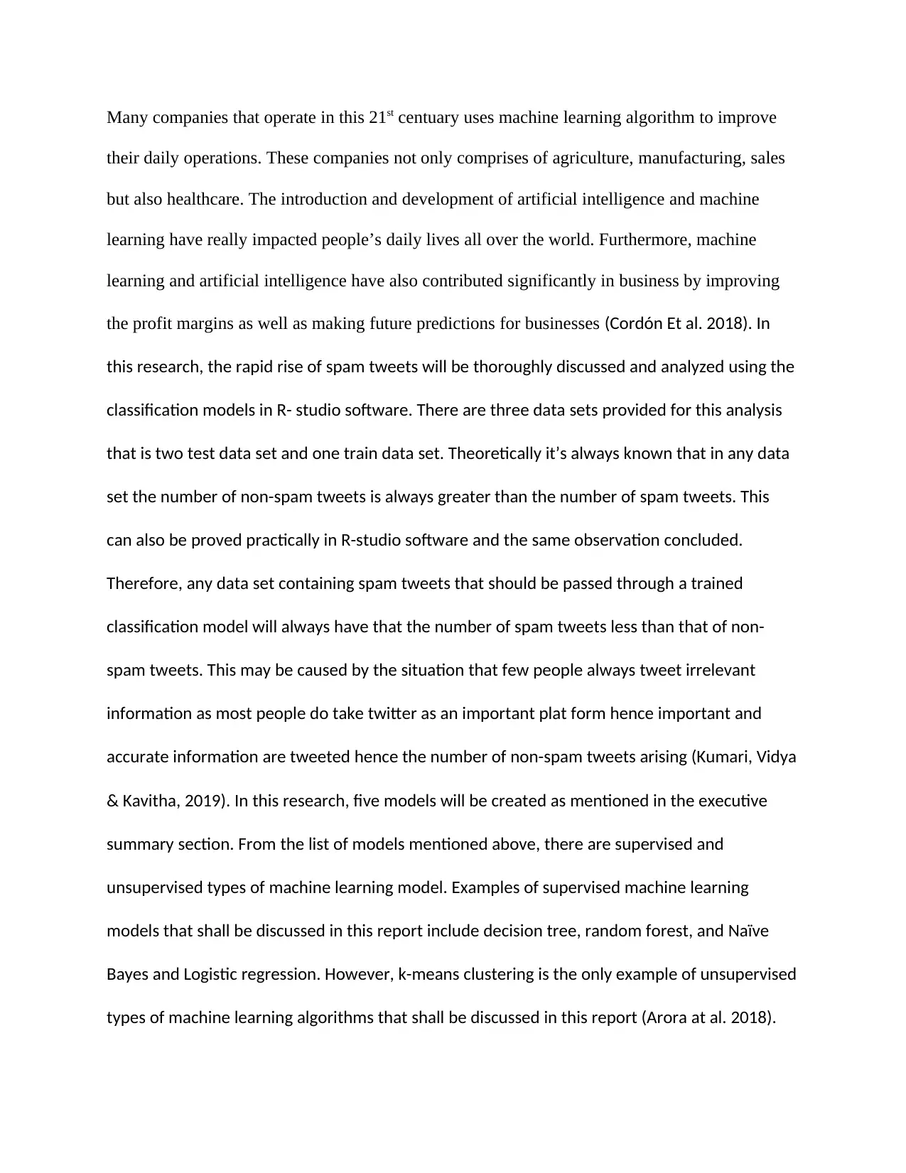
Starting with the logistic regression model, all the three CSV converted datasets will be loaded
on to an R script and then cleaning will be done but after the loading of the necessary tools that
are required for this. The exhibit 1 below shows the loading of the train data and the loading the
tools package that aid in the manipulation of data sets;

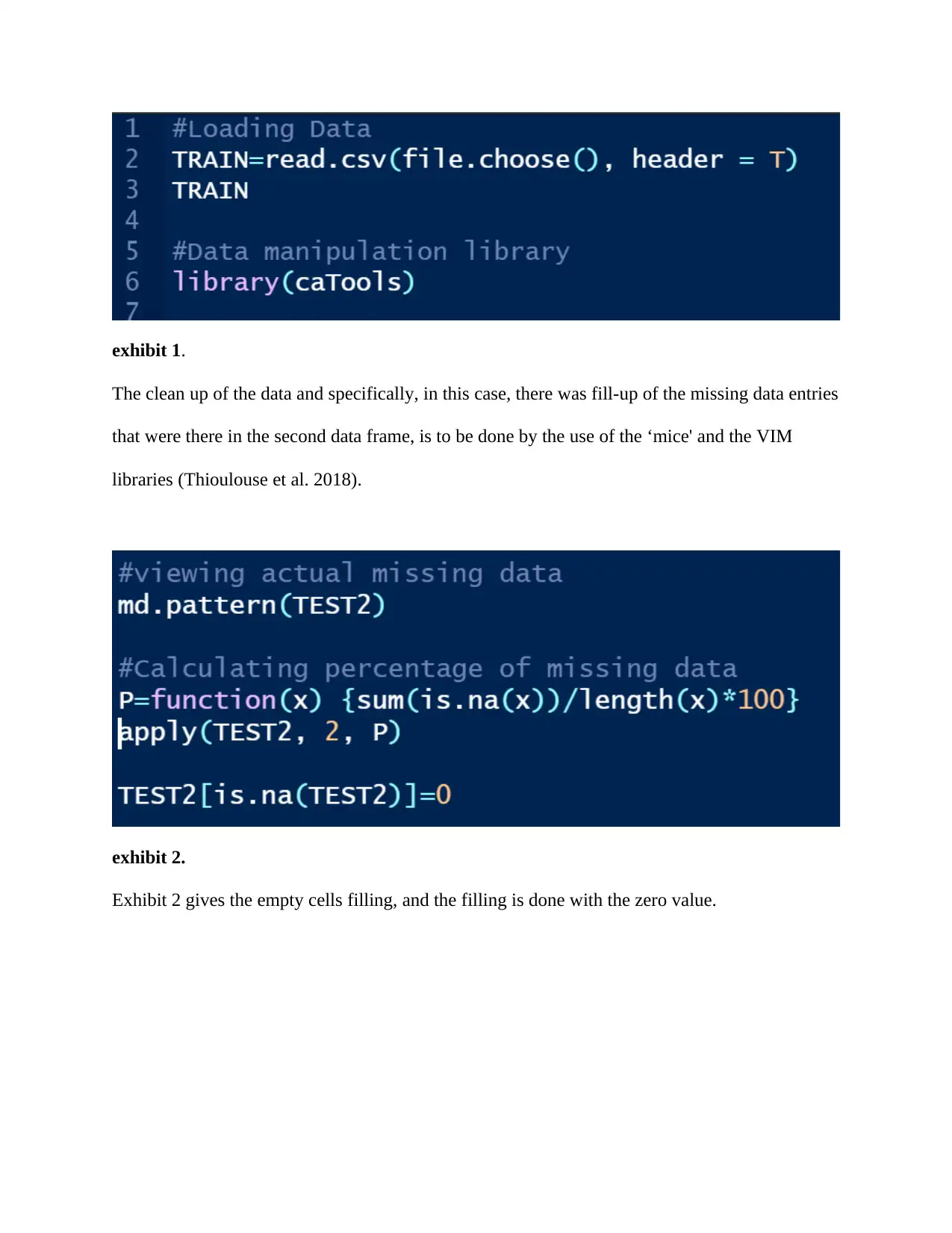
exhibit 1.
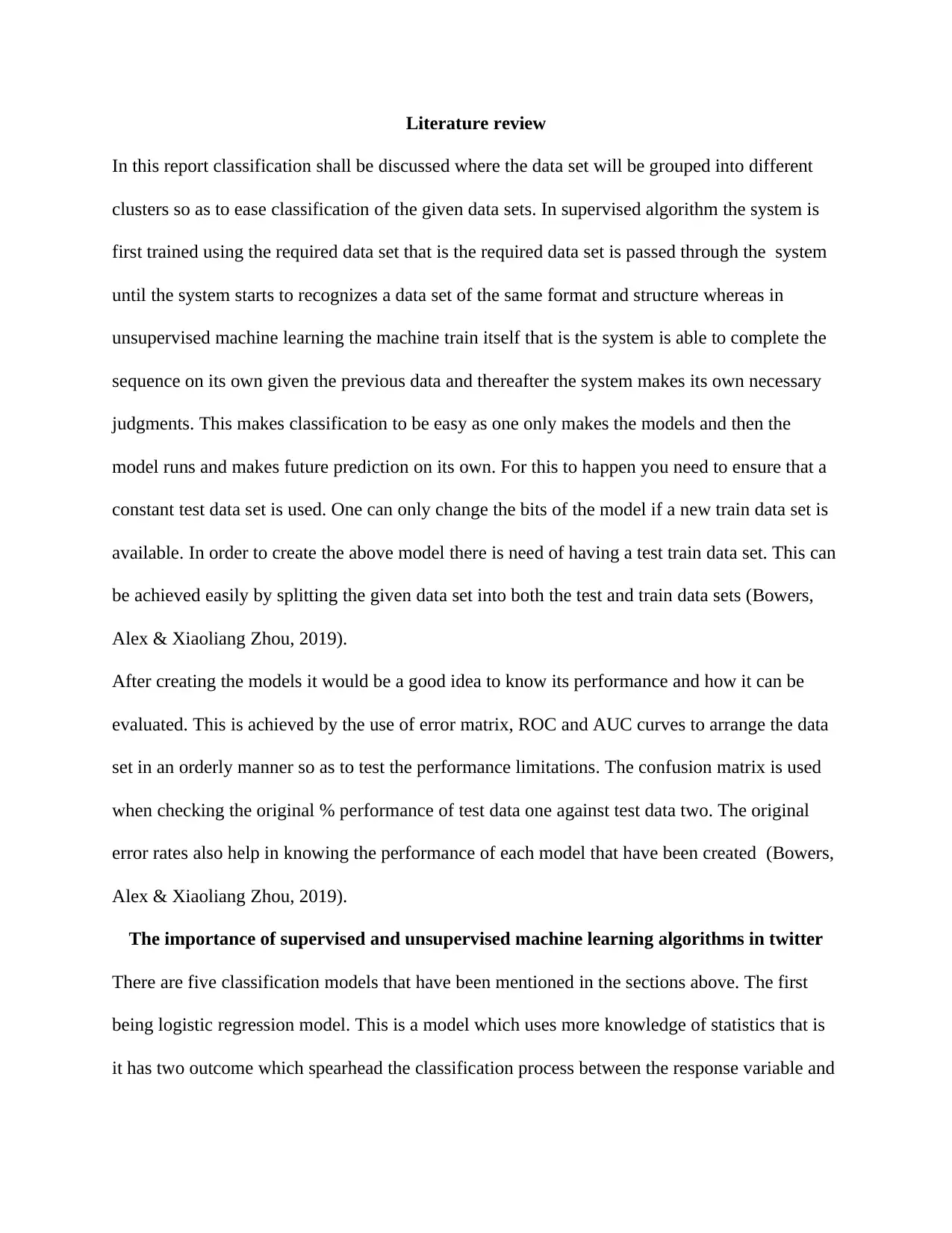
The clean up of the data and specifically, in this case, there was fill-up of the missing data entries
that were there in the second data frame, is to be done by the use of the ‘mice' and the VIM
libraries (Thioulouse et al. 2018).
exhibit 2.
Exhibit 2 gives the empty cells filling, and the filling is done with the zero value.

Exhibit 3.
Exhibit 3 gives the modlog which is the name of the developed model which is done by the use
of the TRAIN data(train set). The actual prediction of the model to follows in the next
subheading where the test datasets are used for making predictions. The accuracy value is used to
check the accuracy of the model at different thresholds. And the accuracy values are gotten by
actually dividing the main diagonal of the confusion matrix by all the matrix values combined to
together (Rodrigues et al. 2018).

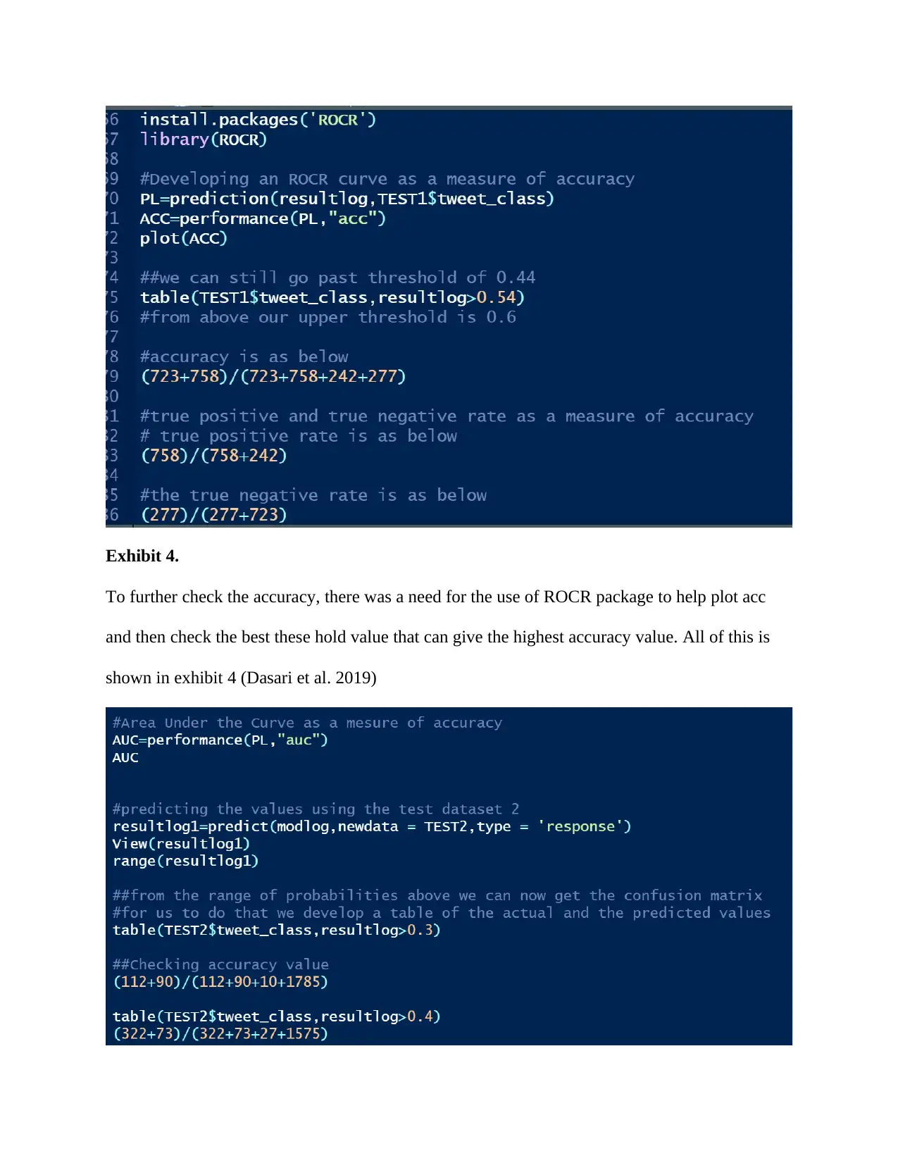
Exhibit 4.
To further check the accuracy, there was a need for the use of ROCR package to help plot acc
and then check the best these hold value that can give the highest accuracy value. All of this is
shown in exhibit 4 (Dasari et al. 2019)

Exhibit 5.
Exhibit 5 gives the actual picture of the areas under the curve command where we are able to
plot and use the area under the curve to check for the models accuracy and it is very clear that the
closer the area under the curve (AUC) is to 1 the stronger, the better and the more accurate the
model is close to 1 (Yamaguchi et al. 2018).
Performance evaluation
For this part, there will be an explanation of the performance of every model and the evaluation
matrix. For the logistic regression, the confusion matrix is of great importance in testing the
accuracy and therefore needs to actually be focused on the most and in this case, after the
prediction of the first test data set, then when the confusion matrix is printed, then it is clear to
see the fact that the accuracy increases with the increase in the threshold value.
The only way to get the maximum to a thresh-hold value that suffices and that gives the highest
degree of accuracy is by the use of the ROCR package that helps in drawing the ROC graph.

On the thresh hold of 0.54, as can be seen from the graph above that has more accuracy as
around 0.5 onwards, there will be the performance of up to 74% which is the highest. This
indicates good performance of the actual model. The AUC which is the area under the curve
stands at 72%. This is closer to 1 and hence high performance.
Conclusion
All the classification models have been developed and then the models used to make predictions
by the use of the evaluation matrices such as the confusion matrix, true positive rate, true
negative rate, ROC, AUC among others. For the models that did not meet the evaluation thresh
holds, there were respective measures that were taken to make sure that they met the
performance threshold. Such measures included pruning of decision trees, reducing classification
trees in a random forest. When pruning and reduction of trees or sample passed through a model
is reduced, then the only guarantee is that the model is bound to improve a great deal.

Bibliography
Arora, Anshul, Sateesh K. Peddoju, Vikas Chouhan, and Ajay Chaudhary. "Poster: Hybrid
Android Malware Detection by Combining Supervised and Unsupervised Learning." In
Proceedings of the 24th Annual International Conference on Mobile Computing and Networking,
pp. 798-800. ACM, 2018.

Bowers, Alex J., and Xiaoliang Zhou. "Receiver operating characteristic (ROC) area under the
curve (AUC): A diagnostic measure for evaluating the accuracy of predictors of education
outcomes." Journal of Education for Students Placed at Risk (JESPAR) 24, no. 1 (2019): 20-46.
Chen, Wei, Shuai Zhang, Renwei Li, and Himan Shahabi. "Performance evaluation of the GIS-
based data mining techniques of best-first decision tree, random forest, and naïve Bayes tree for
landslide susceptibility modeling." Science of the total environment 644 (2018): 1006-1018.
Cordón, Ignacio, Salvador García, Alberto Fernández, and Francisco Herrera. "Imbalance:
oversampling algorithms for imbalanced classification in R." Knowledge-Based Systems 161
(2018): 329-341.
Dasari, Bobby VM, James Hodson, Robert P. Sutcliffe, Ravi Marudanayagam, Keith J. Roberts,
Manuel Abradelo, Paolo Muiesan, Darius F. Mirza, and John Isaac. "Developing and validating a
preoperative risk score to predict 90‐day mortality after liver resection." Journal of surgical
oncology 119, no. 4 (2019): 472-478.
Gelman, Andrew, Ben Goodrich, Jonah Gabry, and Aki Vehtari. "R-squared for Bayesian
regression models." The American Statistician (2019): 1-7.
Kumari, KR Vidya, and C. R. Kavitha. "Spam Detection Using Machine Learning in R." In
International Conference on Computer Networks and Communication Technologies, pp. 55-64.
Springer, Singapore, 2019.