Control Systems: Analysis and Design of Closed Loop Liquid Level

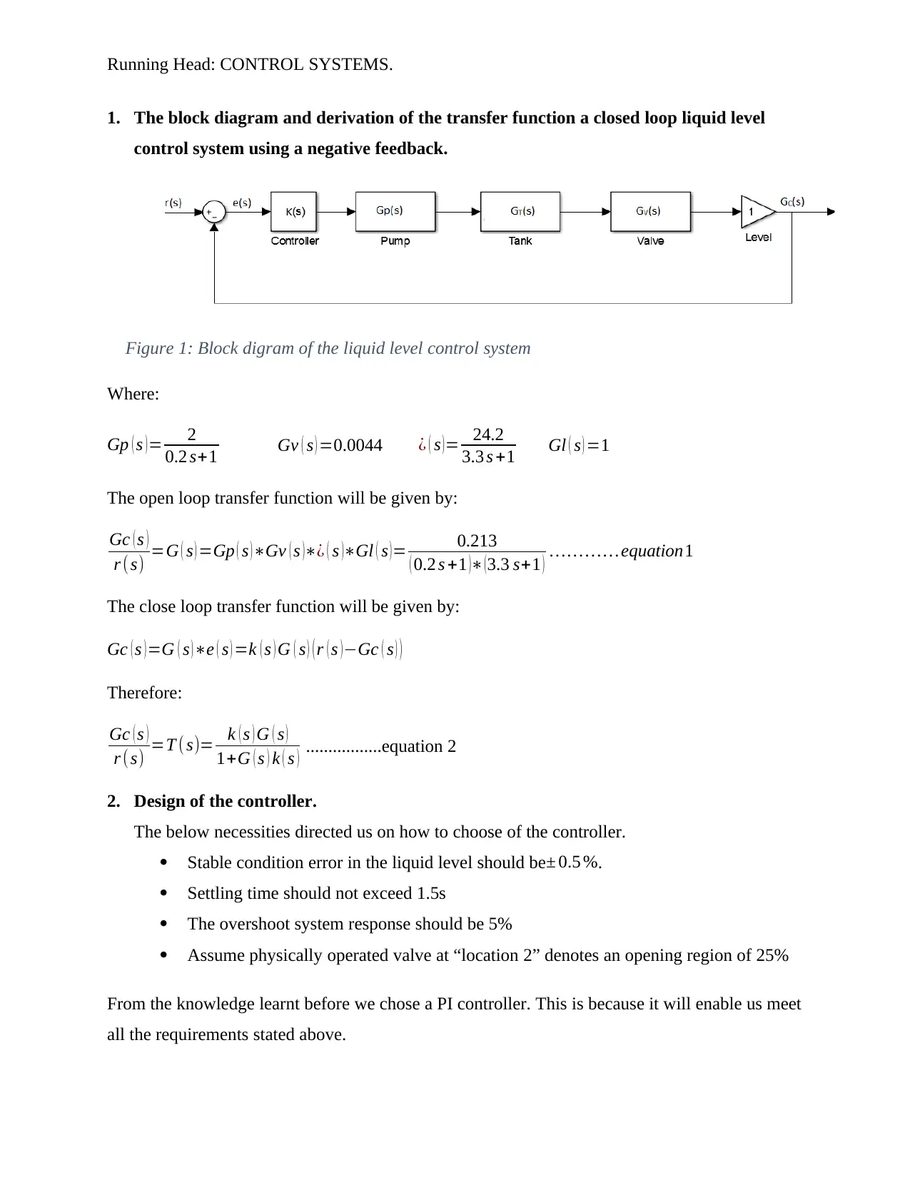
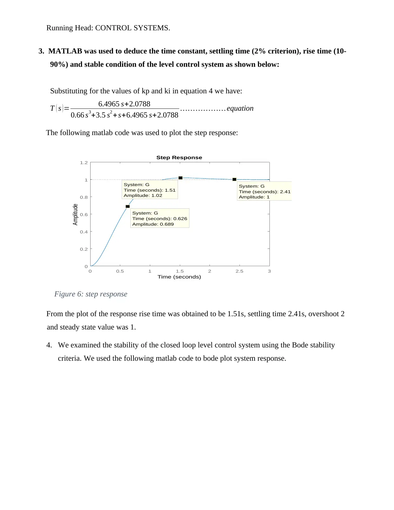
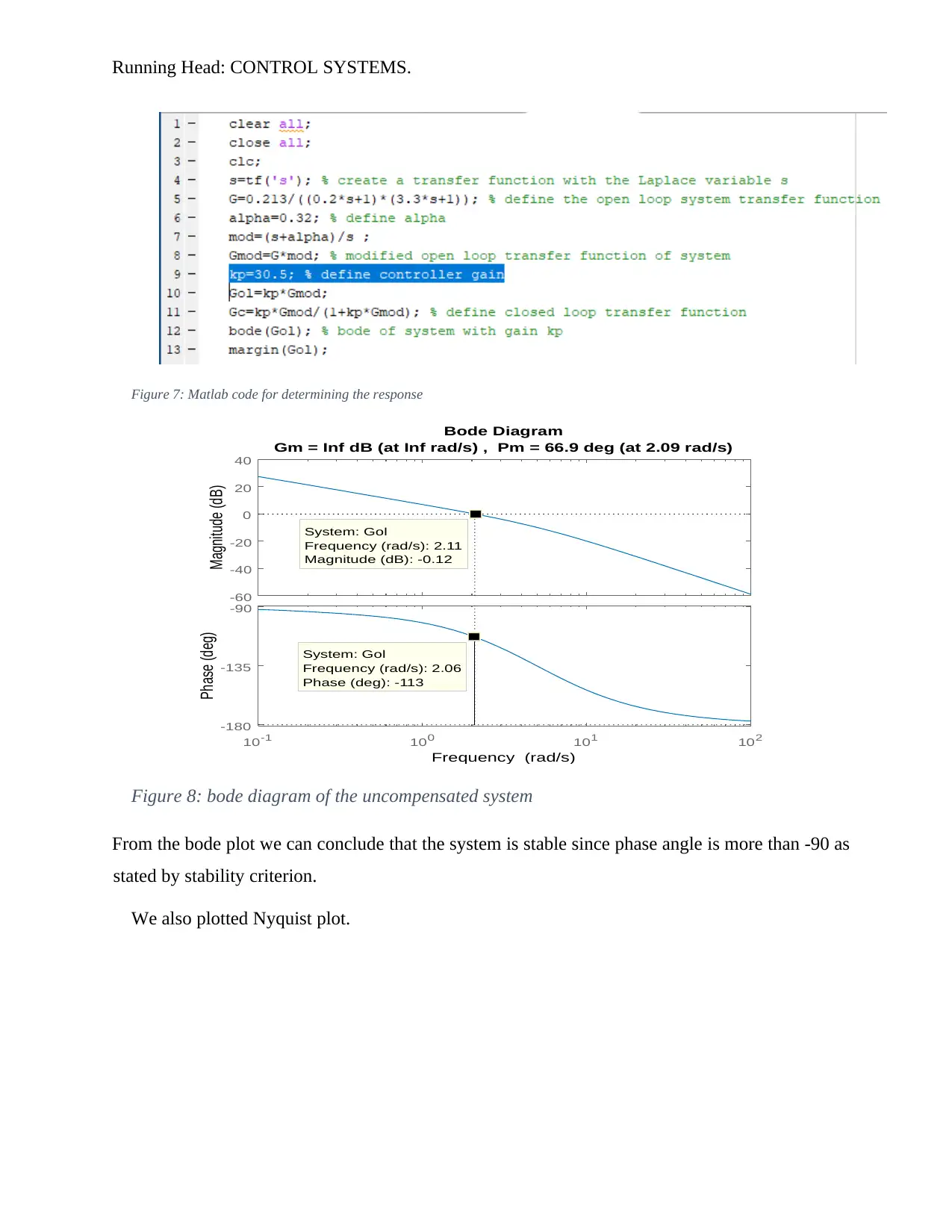
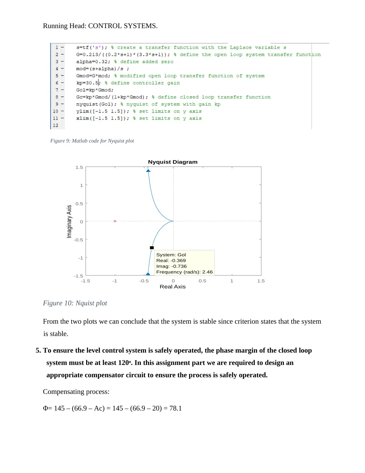
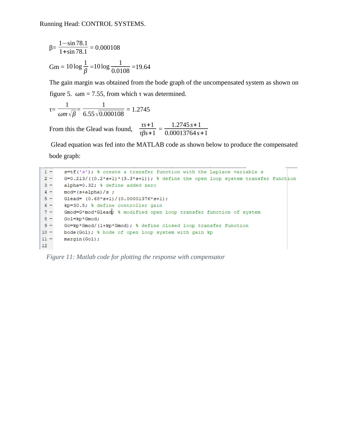
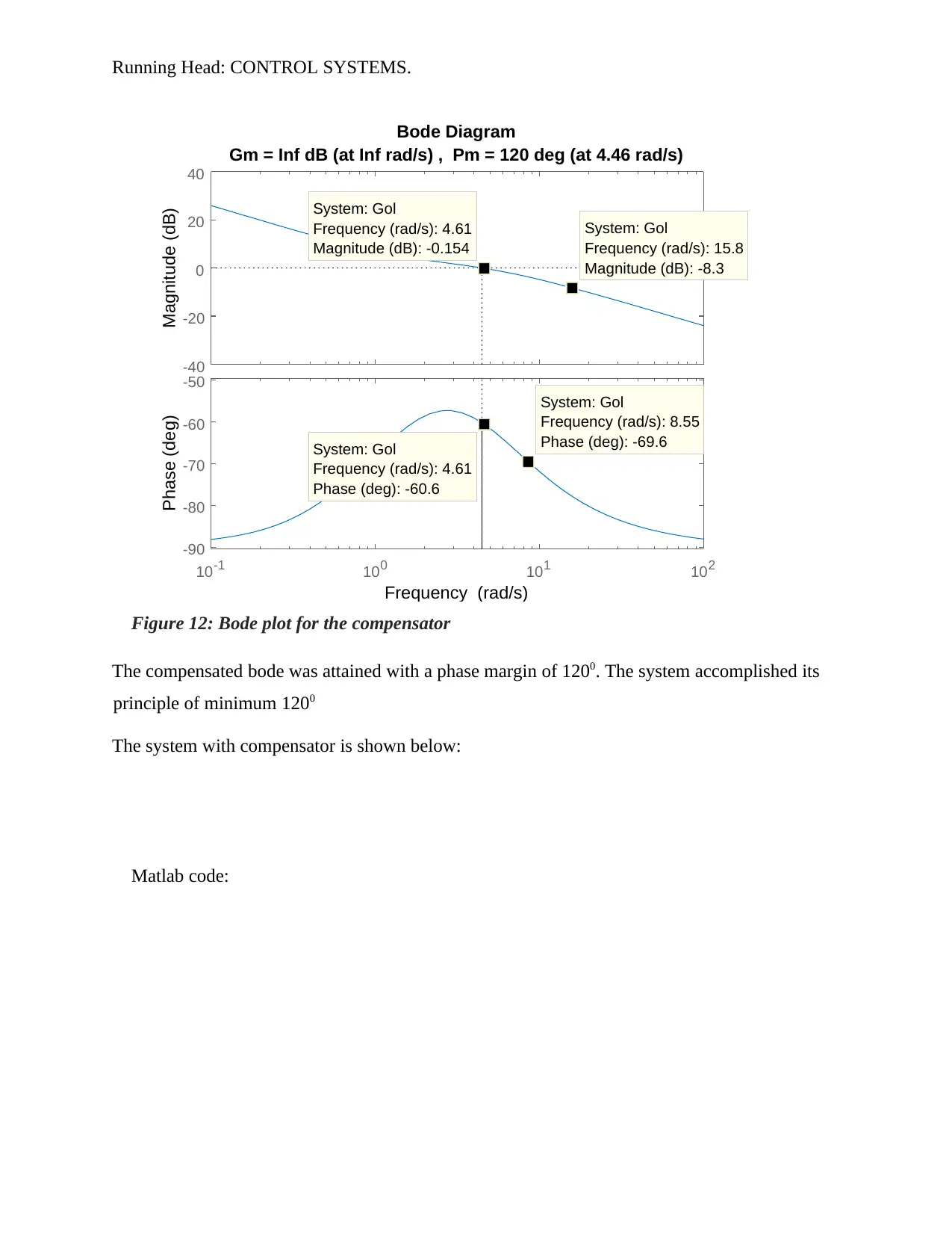
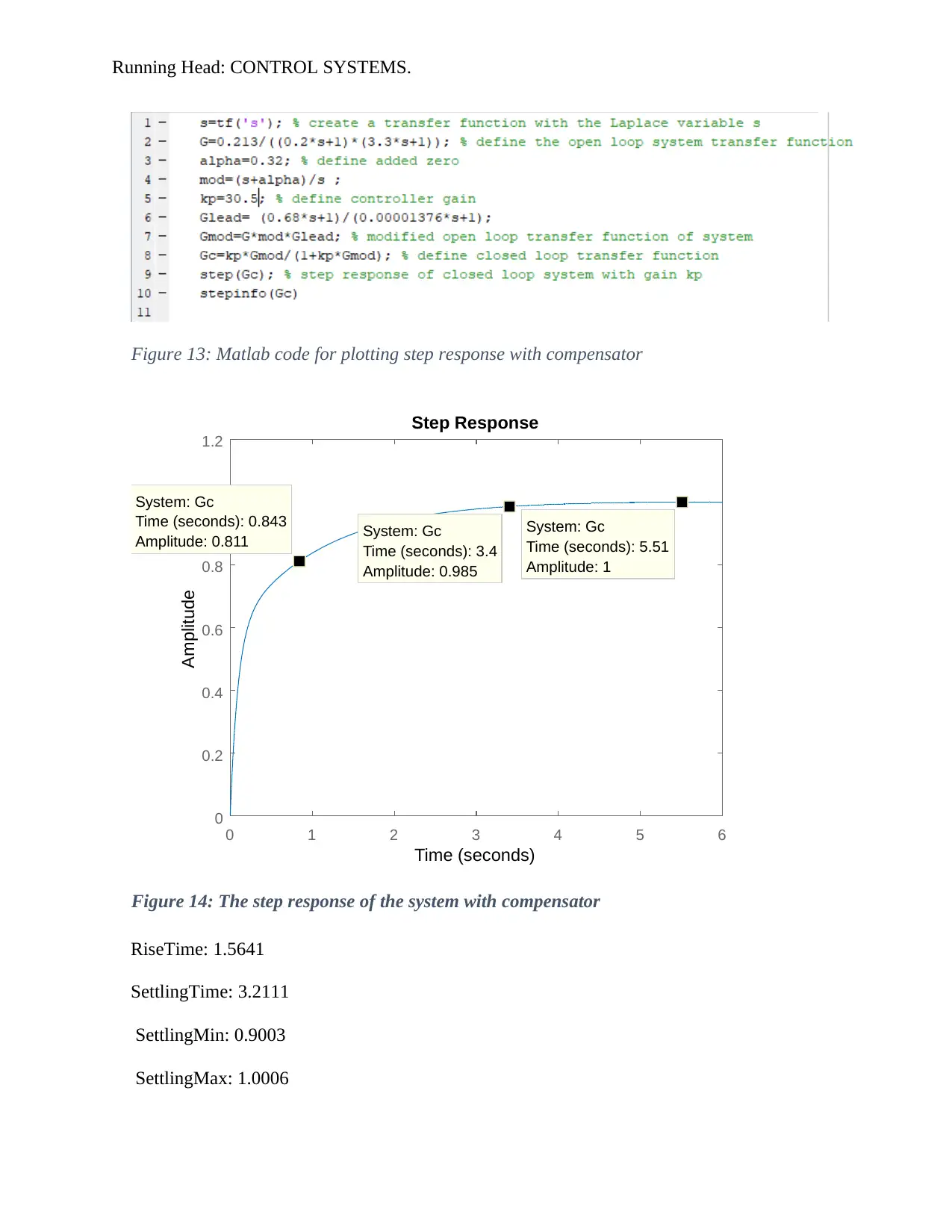
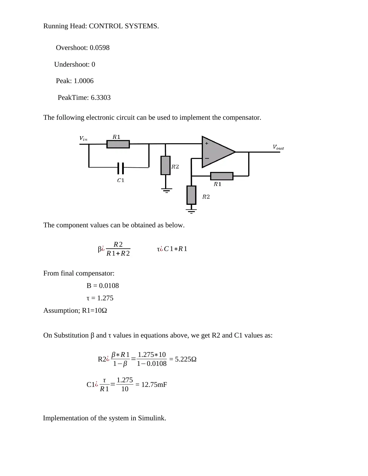
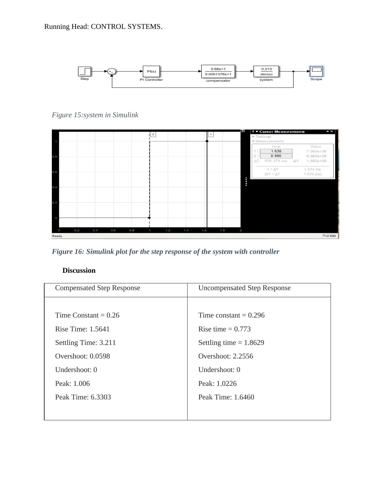
This report presents the design and analysis of a closed-loop liquid level control system using negative feedback. It includes the derivation of the transfer function, controller design with a PI controller to meet specific performance requirements (stable condition error, settling time, and overshoot), and stability analysis using Bode plots and Nyquist plots. The design incorporates MATLAB simulations for root locus analysis, step response evaluation, and compensator design to ensure safe operation with a phase margin of at least 120 degrees. The report also compares the performance of compensated and uncompensated systems, concluding that the compensator improves overshoot and time constant while slightly increasing rise and settling times. Finally, it provides an electronic circuit implementation of the compensator and a Simulink model of the entire system.

Running Head: CONTROL SYSTEMS.
1. The block diagram and derivation of the transfer function a closed loop liquid level
control system using a negative feedback.
Figure 1: Block digram of the liquid level control system
Where:
Gp ( s )= 2
0.2 s+1 Gv ( s ) =0.0044 ¿ ( s )= 24.2
3.3 s +1 Gl ( s ) =1
The open loop transfer function will be given by:
Gc ( s )
r ( s) =G ( s ) =Gp ( s )∗Gv ( s )∗¿ ( s )∗Gl ( s )= 0.213
( 0.2 s +1 )∗ (3.3 s+1 ) … … … … equation1
The close loop transfer function will be given by:
Gc ( s )=G ( s )∗e ( s ) =k ( s ) G ( s ) ( r ( s )−Gc ( s ) )
Therefore:
Gc ( s )
r ( s) =T ( s)= k ( s ) G ( s )
1+G ( s ) k ( s ) .................equation 2
2. Design of the controller.
The below necessities directed us on how to choose of the controller.
 Stable condition error in the liquid level should be ± 0.5 %.
 Settling time should not exceed 1.5s
 The overshoot system response should be 5%
 Assume physically operated valve at “location 2” denotes an opening region of 25%
From the knowledge learnt before we chose a PI controller. This is because it will enable us meet
all the requirements stated above.

Running Head: CONTROL SYSTEMS.
Design procedure for the controller.
kp ( s )=kp+ ki
s
Substituting for G(s) in equation 1
We have our closed loop transfer function as:
T ( s )=
k ( s )∗
[ 0.213
( 0.2 s+1 )∗( 3.3 s +1 ) ]
1+{k ( s )∗
[ 0.213
( 0.2 s+1 )∗ ( 3.3 s+1 ) ]…………………equation 3
Substituting for k ( s ) and solving the equation we have:
T ( s ) = 0.213 skp+ 0.213 ki
0.66 s3+3.5 s2 +s+0.213 skp+0.213 ki ……………………equation 4
We obtained the value of Alpha (𝛼) in order to obtain Kp and Ki for a stable system as follows:
From equation 1 open loop transfer function, G(s) = 0.213
0.66 s2+ 3.5 s+1
Finding the poles using the following quadratic equation:
−b ± √b2−4 ac
2a
−3.5 ± √ 3.52−(4∗0.66∗1)
2∗0.66
Pole 1, P1 = −3.5+ √3.52−(4∗0.66∗1)
2∗0.66 = -0.3
Pole 2, P2 = −3.5− √ 3.52−(4∗0.66∗1)
2∗0.66 = -5
Alpha, 𝛼 < |P1+P2|
𝛼 < |-0.3+-5|

Running Head: CONTROL SYSTEMS.
𝛼 < 5.3
Value of 𝛼 chosen should not exceed summation of poles of the exposed loop system, the
system turns into a stable condition at all values of 𝐾𝑝 the value of alpha was selected to be 0.8.
The integral gain can be defined in terms of proportional gain aski= K p (s+ α )
s .
The values of kp and ki were obtained by plotting the root locus and reading the gain values from
the plot:
Matlab code:
Figure 2: code for calculating root locus
-10 -8 -6 -4 -2 0 2 4 6 8 10
-10
-8
-6
-4
-2
0
2
4
6
8
10
0.34
0.86
0.94
0.64
0.76
0.160.340.50.64
0.76
0.86
0.94
0.985
0.160.5
0.985
2
4
6
8
10
2
4
6
8
10
Root Locus
Real Axis (seconds -1 )
Imaginary Axis (seconds-1 )
System: Gmod
Gain: 30.5
Pole: -2.49 - 1.89i
Damping: 0.797
Overshoot (%): 1.59
Frequency (rad/s): 3.12
Figure 3: Root locus plot
From the figure above the value of kp =30.5 therefore ki=9.76.

Running Head: CONTROL SYSTEMS.
Matlab code for plotting step response.
Figure 4: matlab code for determining step response
The step response is as shown below:
0 0.5 1 1.5 2 2.5 3
0
0.2
0.4
0.6
0.8
1
1.2
Step Response
Time (seconds)
Amplitude
System: Gc
Time (seconds): 1.52
Amplitude: 1.02
System: Gc
Time (seconds): 1.87
Amplitude: 1.02
System: Gc
Time (seconds): 0.314
Amplitude: 0.286
Figure 5:step response settling time=1.7s,percentage overshoot=4%

Running Head: CONTROL SYSTEMS.
3. MATLAB was used to deduce the time constant, settling time (2% criterion), rise time (10-
90%) and stable condition of the level control system as shown below:
Substituting for the values of kp and ki in equation 4 we have:
T ( s ) = 6.4965 s+2.0788
0.66 s3+3.5 s2 + s+6.4965 s+2.0788 … … … … … … equation
The following matlab code was used to plot the step response:
0 0.5 1 1.5 2 2.5 3
0
0.2
0.4
0.6
0.8
1
1.2
Step Response
Time (seconds)
Amplitude
System: G
Time (seconds): 2.41
Amplitude: 1
System: G
Time (seconds): 1.51
Amplitude: 1.02
System: G
Time (seconds): 0.626
Amplitude: 0.689
Figure 6: step response
From the plot of the response rise time was obtained to be 1.51s, settling time 2.41s, overshoot 2
and steady state value was 1.
4. We examined the stability of the closed loop level control system using the Bode stability
criteria. We used the following matlab code to bode plot system response.

Running Head: CONTROL SYSTEMS.
Figure 7: Matlab code for determining the response
-60
-40
-20
0
20
40
Magnitude (dB)
10 -1 10 0 10 1 10 2
-180
-135
-90
Phase (deg)
Bode Diagram
Gm = Inf dB (at Inf rad/s) , Pm = 66.9 deg (at 2.09 rad/s)
Frequency (rad/s)
System: Gol
Frequency (rad/s): 2.11
Magnitude (dB): -0.12
System: Gol
Frequency (rad/s): 2.06
Phase (deg): -113
Figure 8: bode diagram of the uncompensated system
From the bode plot we can conclude that the system is stable since phase angle is more than -90 as
stated by stability criterion.
We also plotted Nyquist plot.

Running Head: CONTROL SYSTEMS.
Figure 9: Matlab code for Nyquist plot
-1.5 -1 -0.5 0 0.5 1 1.5
-1.5
-1
-0.5
0
0.5
1
1.5
Nyquist Diagram
Real Axis
Imaginary Axis
System: Gol
Real: -0.369
Imag: -0.736
Frequency (rad/s): 2.46
Figure 10: Nquist plot
From the two plots we can conclude that the system is stable since criterion states that the system
is stable.
5. To ensure the level control system is safely operated, the phase margin of the closed loop
system must be at least 120ᵒ. In this assignment part we are required to design an
appropriate compensator circuit to ensure the process is safely operated.
Compensating process:
Φ= 145 – (66.9 – Ac) = 145 – (66.9 – 20) = 78.1

Running Head: CONTROL SYSTEMS.
β= 1−sin 78.1
1+sin 78.1 = 0.000108
Gm = 10 log 1
β =10 log 1
0.0108 =19.64
The gain margin was obtained from the bode graph of the uncompensated system as shown on
figure 5. ωm = 7.55, from which τ was determined.
τ= 1
ωm √β = 1
6.55 √ 0.000108 = 1.2745
From this the Glead was found, τs+1
τβs+1 = 1.2745 s+ 1
0.00013764 s +1
Glead equation was fed into the MATLAB code as shown below to produce the compensated
bode graph:
Figure 11: Matlab code for plotting the response with compensator

Running Head: CONTROL SYSTEMS.
-40
-20
0
20
40
Magnitude (dB)
10-1 100 101 102
-90
-80
-70
-60
-50
Phase (deg)
Bode Diagram
Gm = Inf dB (at Inf rad/s) , Pm = 120 deg (at 4.46 rad/s)
Frequency (rad/s)
System: Gol
Frequency (rad/s): 4.61
Magnitude (dB): -0.154
System: Gol
Frequency (rad/s): 4.61
Phase (deg): -60.6
System: Gol
Frequency (rad/s): 15.8
Magnitude (dB): -8.3
System: Gol
Frequency (rad/s): 8.55
Phase (deg): -69.6
Figure 12: Bode plot for the compensator
The compensated bode was attained with a phase margin of 1200. The system accomplished its
principle of minimum 1200
The system with compensator is shown below:
Matlab code:

Running Head: CONTROL SYSTEMS.
Figure 13: Matlab code for plotting step response with compensator
0 1 2 3 4 5 6
0
0.2
0.4
0.6
0.8
1
1.2
Step Response
Time (seconds)
Amplitude
System: Gc
Time (seconds): 5.51
Amplitude: 1
System: Gc
Time (seconds): 3.4
Amplitude: 0.985
System: Gc
Time (seconds): 0.843
Amplitude: 0.811
Figure 14: The step response of the system with compensator
RiseTime: 1.5641
SettlingTime: 3.2111
SettlingMin: 0.9003
SettlingMax: 1.0006

Running Head: CONTROL SYSTEMS.
Overshoot: 0.0598
Undershoot: 0
Peak: 1.0006
PeakTime: 6.3303
The following electronic circuit can be used to implement the compensator.
The component values can be obtained as below.
β¿ R 2
R 1+ R 2 τ¿ C 1∗R 1
From final compensator:
Β = 0.0108
τ = 1.275
Assumption; R1=10Ω
On Substitution β and τ values in equations above, we get R2 and C1 values as:
R2¿ β∗R 1
1−β = 1.275∗10
1−0.0108 = 5.225Ω
C1¿ τ
R 1 = 1.275
10 = 12.75mF
Implementation of the system in Simulink.

Running Head: CONTROL SYSTEMS.
Figure 15:system in Simulink
Figure 16: Simulink plot for the step response of the system with controller
Discussion
Compensated Step Response Uncompensated Step Response
Time Constant = 0.26
Rise Time: 1.5641
Settling Time: 3.211
Overshoot: 0.0598
Undershoot: 0
Peak: 1.006
Peak Time: 6.3303
Time constant = 0.296
Rise time = 0.773
Settling time = 1.8629
Overshoot: 2.2556
Undershoot: 0
Peak: 1.0226
Peak Time: 1.6460

Running Head: CONTROL SYSTEMS.
From the table above it can be seen the overshoot for the compensated system is quite low
compared to that of uncompensated system. We can also conclude that the peak value for the
compensated system is also small. Therefore a compensated controller has a better performance
compared to uncompensated.
Conclusion:
From the assignment we can conclude that the comparison between the compensated step
response values and uncompensated step response values illustrates that by adding compensators
the overshoot of a system is controlled (eliminated) and time constant has been improved.
However, the rise time and settling time has increased with the adding of the compensators. In
conclusion, the lab assignment was successful.