2018 Griffith University Coastal Engineering Assignment: Simple Models
VerifiedAdded on 2023/06/10
|13
|2158
|360
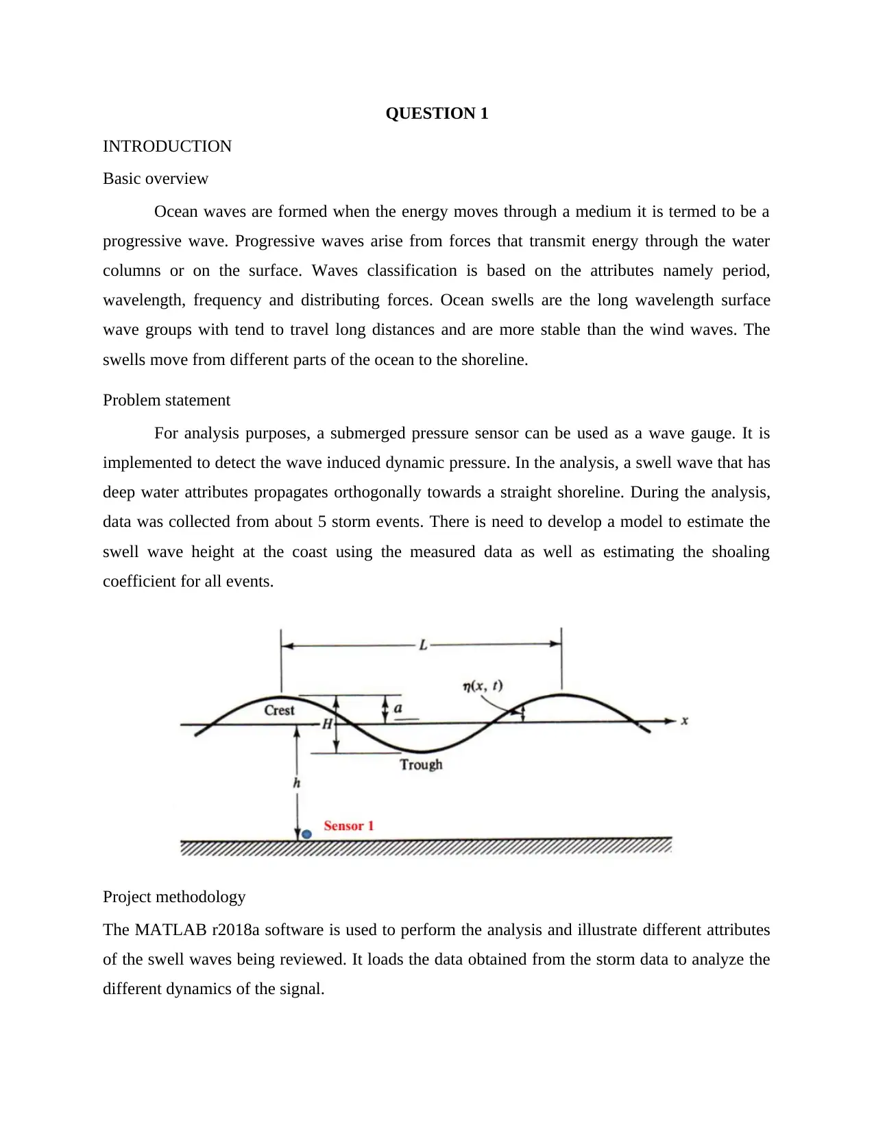
Project
AI Summary
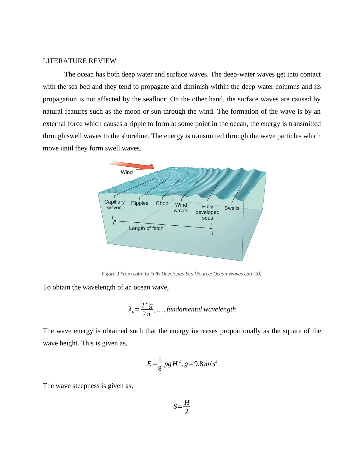
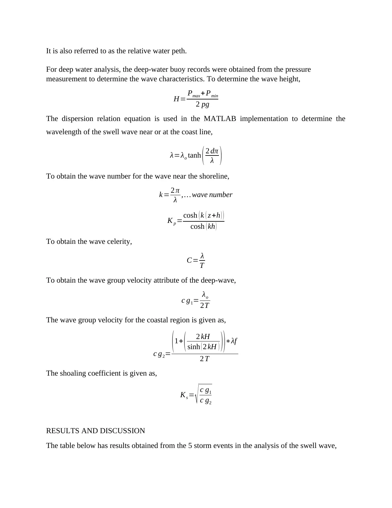
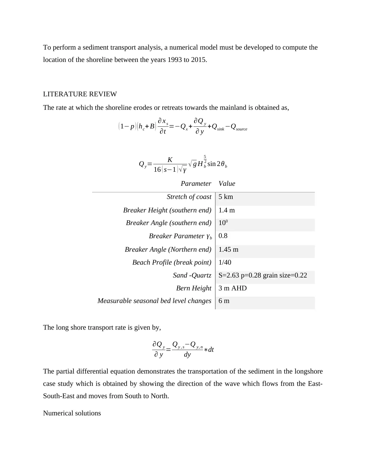
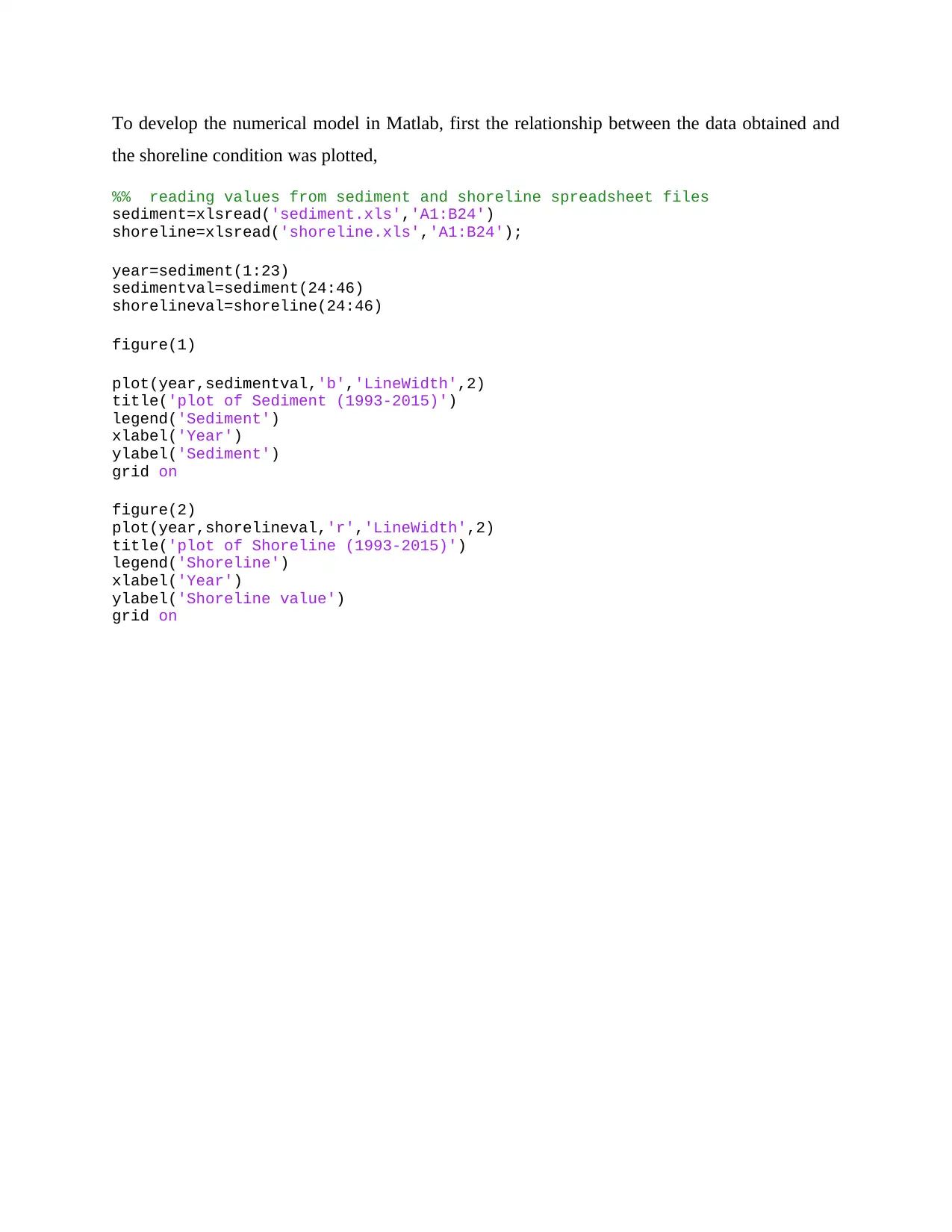
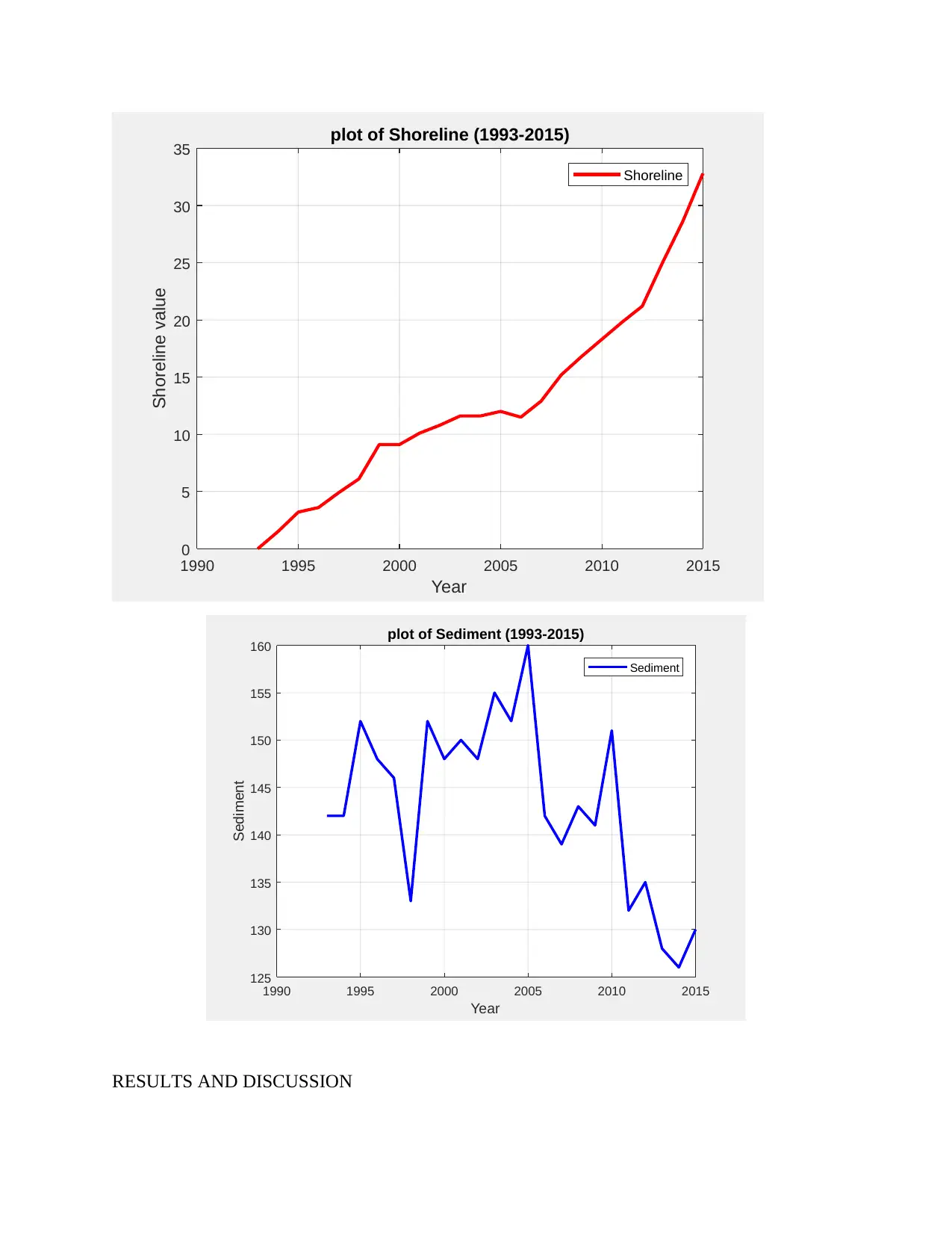
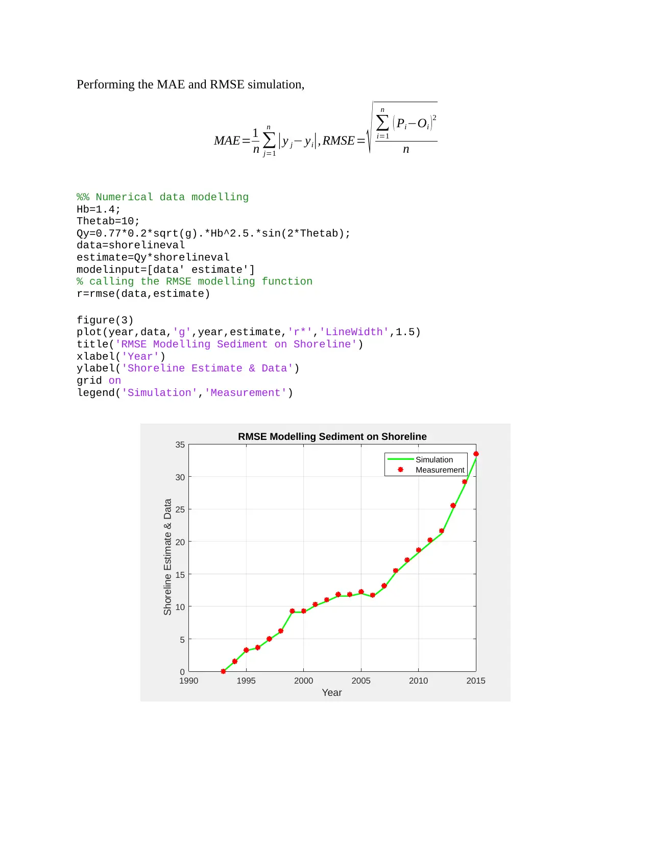
This assignment addresses two key aspects of coastal engineering. Question 1 focuses on developing a model to estimate swell wave height at the coast using data from a submerged pressure sensor and calculating the shoaling coefficient for five storm events. The analysis utilizes MATLAB to process wave characteristics like wave height, wavelength, and wave celerity, and includes graphical illustrations of relative water depth and shoaling coefficients. Question 2 involves analyzing sediment transport rates and shoreline changes between 1993 and 2015. A numerical model is developed using MATLAB to simulate shoreline positions, incorporating data from sediment transport and aerial views. The model calculates the root mean square error (RMSE) and plots sediment and shoreline trends, offering insights into coastal erosion and sediment dynamics. The report concludes with a discussion of the MATLAB software's efficiency in coastal engineering modeling.
1 out of 13


Your All-in-One AI-Powered Toolkit for Academic Success.
+13062052269
info@desklib.com
Available 24*7 on WhatsApp / Email
![[object Object]](/_next/static/media/star-bottom.7253800d.svg)
Copyright © 2020–2026 A2Z Services. All Rights Reserved. Developed and managed by ZUCOL.