Major Assignment Part 1: Linear and Log-Log Model Analysis (ECON 301)

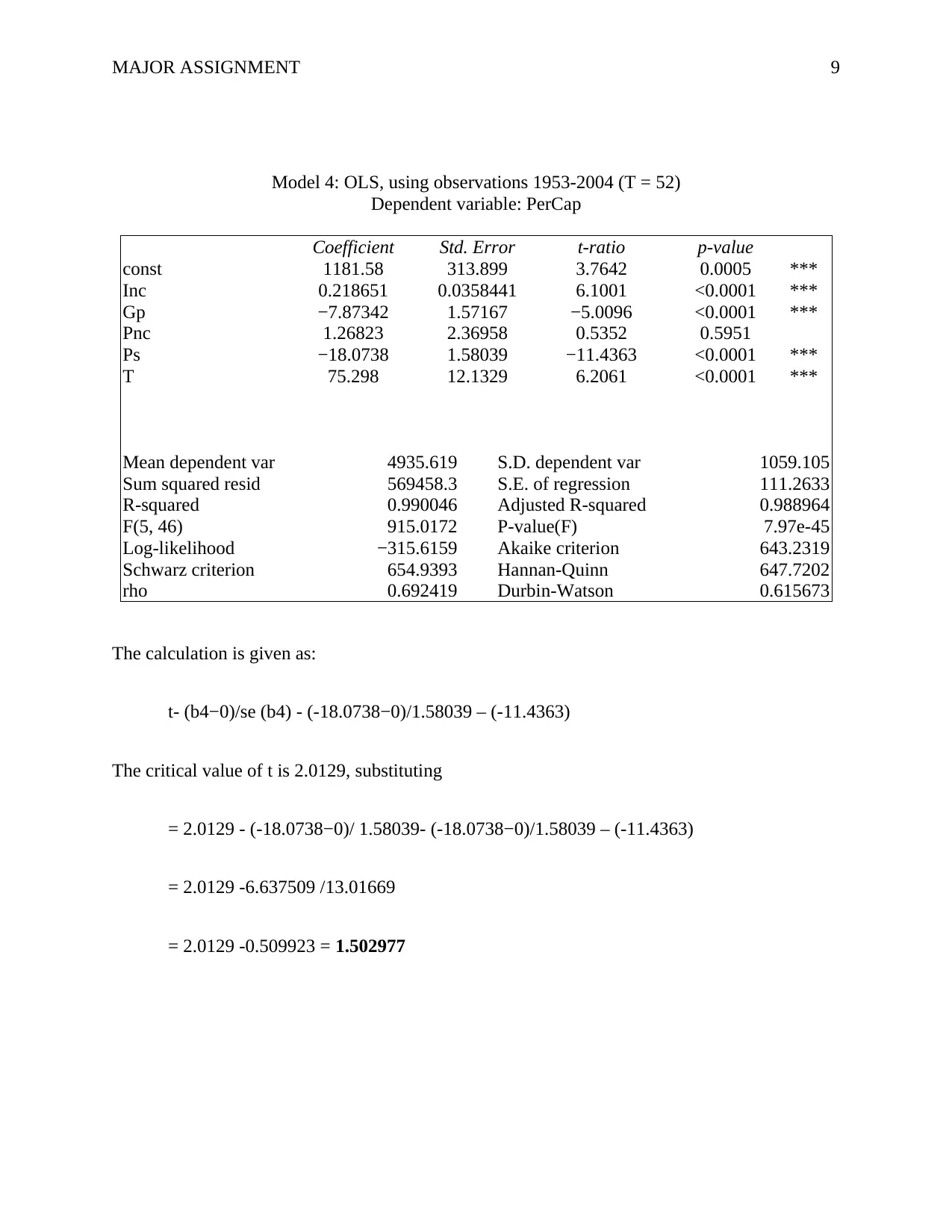
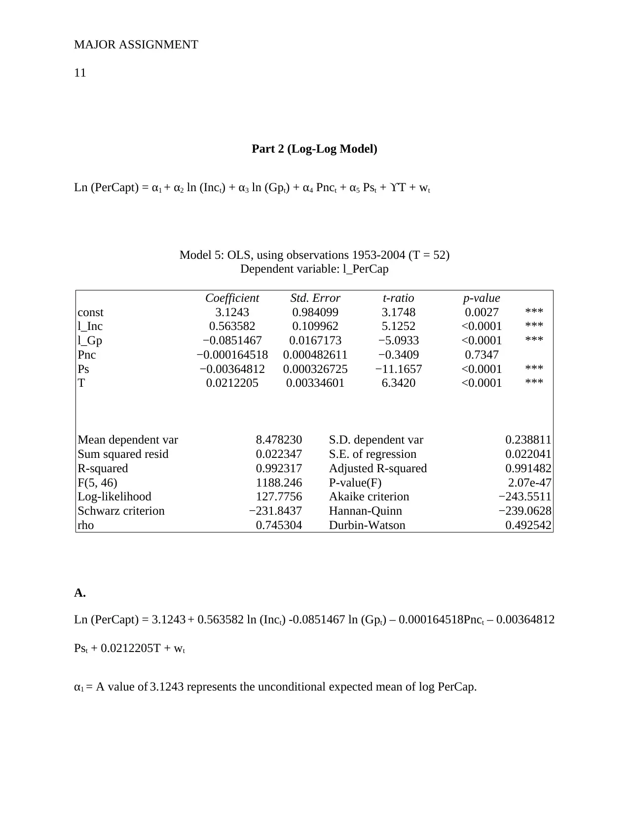
This assignment presents a detailed analysis of two regression models: a linear model and a log-log model, focusing on per capita gas consumption. The solution includes the output of Ordinary Least Squares (OLS) regressions, coefficient interpretations, and statistical tests for significance. The student calculates price and income elasticities of gas consumption, tests hypotheses, and evaluates the overall significance of parameters. The assignment further explores a log-log model, interpreting its coefficients and constructing confidence intervals. Finally, the student compares the two models, providing a critical evaluation of their strengths and weaknesses, and explaining why the linear regression model is preferred based on econometric principles and economic interpretations. The document showcases a comprehensive understanding of regression analysis and its application in economics.

Running head: MAJOR ASSIGNMENT 1
Major Assignment
Name:
Institutional Affiliation:

MAJOR ASSIGNMENT 2
Major Assignment
Part 1 (Linear Model)
A.
Model 4: OLS, using observations 1953-2004 (T = 52)
Dependent variable: PerCap
Coefficient Std. Error t-ratio p-value
const 1181.58 313.899 3.7642 0.0005 ***
Inc 0.218651 0.0358441 6.1001 <0.0001 ***
Gp −7.87342 1.57167 −5.0096 <0.0001 ***
Pnc 1.26823 2.36958 0.5352 0.5951
Ps −18.0738 1.58039 −11.4363 <0.0001 ***
T 75.298 12.1329 6.2061 <0.0001 ***
Mean dependent var 4935.619 S.D. dependent var 1059.105
Sum squared resid 569458.3 S.E. of regression 111.2633
R-squared 0.990046 Adjusted R-squared 0.988964
F(5, 46) 915.0172 P-value(F) 7.97e-45
Log-likelihood −315.6159 Akaike criterion 643.2319
Schwarz criterion 654.9393 Hannan-Quinn 647.7202
rho 0.692419 Durbin-Watson 0.615673
Therefore, PerCapt = 1181.58 + 0.218651Inct – 7.87342Gpt + 1.26823Pnct – 18.0738Ps +
75.298T +ϵt
Explanation:
Per household gas consumption is positively related to per capital disposable income, inversely
related to the price index for gasoline, positively related to the price index of new cars,

MAJOR ASSIGNMENT 3
negatively associated to the aggregate price index of the consumer services, and positively
related to time trend. When the price index for gasoline increases, per household gas
consumption would decrease and vice versa.
In the same way, when price for new cars rises, the household consumption will also increase,
and vice versa. The rise in the aggregate price for consumer services would also decrease
household gas consumption, and vice versa. The estimated signs of these coefficients do agree
with my expectations. For instance, since cars are a luxury commodity, the price index for new
cars would be expected to be inversely related to household gas consumption.
B.

MAJOR ASSIGNMENT 4
Comment:
From the scatter graph above, it is clear that as per capita disposable income (Inc) increases, per
household gas consumption among consumer increases, because now consumers have huge
disposable incomes to spend on gas. However, any decrease in the per capital disposal increase
would decrease household gas consumption.

MAJOR ASSIGNMENT 5
C.
Using the critical value method to test individual significance of the coefficients of Inc and Gp at
5% significance level
1) Price Index For Gasoline (Gp) Test
The coefficient Inc is 0.218651
Therefore,
lb = Coefficient (Inc) – Critical value of t = 0.218651 – 2.0129 = -1.79425
ub = Coefficient (Inc) + Critical value of t = 0.218651 + 2.0129 = 2.23155
Thus,
-1.79425≤ t ≤2.23155
The t-test for the regression coefficient is statistically significant, since it lies within the range.

MAJOR ASSIGNMENT 6
2) Per Capital Disposable Income (Inc) Test
The coefficient Inc is −7.87342
Therefore,
lb = Coefficient (Inc) – Critical value of t = −7.87342 – 2.0129 = -9.88632
ub = Coefficient (Inc) + Critical value of t = −7.87342 + 2.0129 = -5.86052
-9.88632≤ t ≤-5.86052
The t-test for the regression coefficient is statistically significant, since it lies within the range.

MAJOR ASSIGNMENT 7
D.
Gas price elasticity of per household gas consumption (PerCap) and income elasticity of per
household gas consumption (PerCap) at the sample mean values
1. Price elasticity of per capita gas consumption
Mean Median Minimum Maximum
Inc 16805. 16692. 8685.0 27113.
Gp 51.343 47.502 16.668 123.90
Pnc 87.567 78.800 44.800 141.70
Ps 89.777 64.150 19.400 222.80
T 26.500 26.500 1.0000 52.000
The price elasticity is computed using the following formula
PE = (ΔQuantity/ΔPprice) * (Price/Qquantity)
The (ΔQuantity/ΔPrice) is presented in the above equation by the coefficient – 7.87342.
To determine (Price/Quantity), the mean of price (51.343) is used as well as the mean of Ps
which is 89.777.
Therefore we have Price elasticity = – 7.87342 * 51.343/89.777= -4.50277
This means that an increase in the price by 1 unit will decrease quantity demanded by 4.50277
units.

MAJOR ASSIGNMENT 8
2. Income elasticity of per capita gas consumption
Income elasticity = (ΔQuantity/ΔPprice) * (Price/Qquantity)
The (ΔQuantity/ΔPrice) is presented in the above equation by the coefficient – 7.87342.
To determine (Price/Quantity), the mean of price (51.343) is used as well as the mean of Ps
which is 87.567.
Therefore we have PE = – 7.87342 * 51.343/87.567= -4.616
This means that a decrease in the income by 1 unit will decrease quantity demanded by 4.616
units.
E.
The null hypothesis here is represented as β4 - 0 against its alternative, which is positive; thus
meaning that β4 >0. Therefore, the test statistic is given as follows:
t= (b4−0)/se (b4) ∼ t46
Provided that β4 - 0 (and that the null hypothesis is true), we use the confidence alpha= 0.05;
thus, making the critical value for the one sided alternative (β4>0) equal to 1.686.
From here, the decision rule is not accepting H0 in favor of the H1 if the computed value of t-
statistic is within the rejection region of the test; especially, if it is greater than 1.686.

MAJOR ASSIGNMENT 9
Model 4: OLS, using observations 1953-2004 (T = 52)
Dependent variable: PerCap
Coefficient Std. Error t-ratio p-value
const 1181.58 313.899 3.7642 0.0005 ***
Inc 0.218651 0.0358441 6.1001 <0.0001 ***
Gp −7.87342 1.57167 −5.0096 <0.0001 ***
Pnc 1.26823 2.36958 0.5352 0.5951
Ps −18.0738 1.58039 −11.4363 <0.0001 ***
T 75.298 12.1329 6.2061 <0.0001 ***
Mean dependent var 4935.619 S.D. dependent var 1059.105
Sum squared resid 569458.3 S.E. of regression 111.2633
R-squared 0.990046 Adjusted R-squared 0.988964
F(5, 46) 915.0172 P-value(F) 7.97e-45
Log-likelihood −315.6159 Akaike criterion 643.2319
Schwarz criterion 654.9393 Hannan-Quinn 647.7202
rho 0.692419 Durbin-Watson 0.615673
The calculation is given as:
t- (b4−0)/se (b4) - (-18.0738−0)/1.58039 – (-11.4363)
The critical value of t is 2.0129, substituting
= 2.0129 - (-18.0738−0)/ 1.58039- (-18.0738−0)/1.58039 – (-11.4363)
= 2.0129 -6.637509 /13.01669
= 2.0129 -0.509923 = 1.502977

MAJOR ASSIGNMENT
10
Therefore, given that this value is within the rejection area, it then means that there is sufficient
evidence at the 5 percent level of significance to induce that the null hypothesis is not correct;
therefore, the null hypothesis is not accepted at the 5% level of significance.

MAJOR ASSIGNMENT
11
Part 2 (Log-Log Model)
Ln (PerCapt) = α1 + α2 ln (Inct) + α3 ln (Gpt) + α4 Pnct + α5 Pst + ϒT + wt
Model 5: OLS, using observations 1953-2004 (T = 52)
Dependent variable: l_PerCap
Coefficient Std. Error t-ratio p-value
const 3.1243 0.984099 3.1748 0.0027 ***
l_Inc 0.563582 0.109962 5.1252 <0.0001 ***
l_Gp −0.0851467 0.0167173 −5.0933 <0.0001 ***
Pnc −0.000164518 0.000482611 −0.3409 0.7347
Ps −0.00364812 0.000326725 −11.1657 <0.0001 ***
T 0.0212205 0.00334601 6.3420 <0.0001 ***
Mean dependent var 8.478230 S.D. dependent var 0.238811
Sum squared resid 0.022347 S.E. of regression 0.022041
R-squared 0.992317 Adjusted R-squared 0.991482
F(5, 46) 1188.246 P-value(F) 2.07e-47
Log-likelihood 127.7756 Akaike criterion −243.5511
Schwarz criterion −231.8437 Hannan-Quinn −239.0628
rho 0.745304 Durbin-Watson 0.492542
A.
Ln (PerCapt) = 3.1243 + 0.563582 ln (Inct) -0.0851467 ln (Gpt) – 0.000164518Pnct – 0.00364812
Pst + 0.0212205T + wt
α1 = A value of 3.1243 represents the unconditional expected mean of log PerCap.

MAJOR ASSIGNMENT
12
α2 = A 100 percent change in Inc leads to a 100*0.563582 percentage point change in the
probability that PerCab occurs.
α3 = A 100 percent change in Inc leads to a 100*0.0851467 percentage point change in the
probability that PerCab occurs
α4 = the movement of 0.000164518 from 0 to 1 produces a 100*0.000164518 percent point
change in the probability that PerCab occurs
α5 = the movement of 0.00364812 from 0 to 1 produces a 100*0.00364812 percent point change
in the probability that PerCab occurs
B.
To calculate the 99% confidence interval for ln (Gpt), I will use the following parameters;
Number of predictors = 5
Regression coefficient of ln (Gpt) = -0.0851
Sample size = 52
Standard error of ln (Gpt) = 0.01671
Therefore,
99% confidence interval for ln (Gpt): -0.13000 ≤ α ≤ -0.04020
C.