Electrical and Electronic Principles - Complex Waveforms TMA Solution

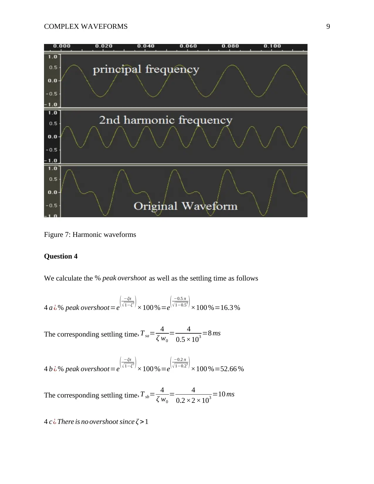
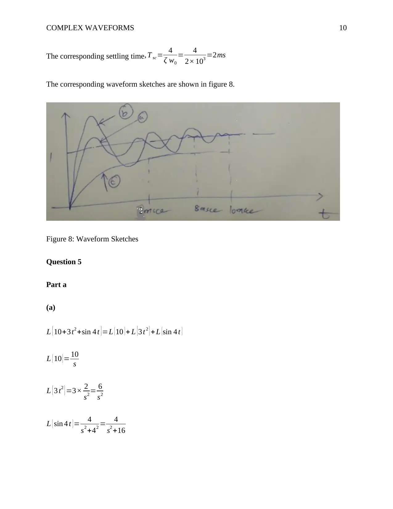
This document presents a comprehensive solution to a complex waveforms and transients assignment in R-L-C circuits. The solution begins with definitions of even and odd functions, as well as half-wave symmetry, crucial for understanding Fourier series applications. It then addresses the analysis of waveforms, including the determination of Fourier series coefficients for specific waveforms and the impact of distortions on harmonic content. The assignment delves into frequency analysis using Fourier transforms, identifying principle frequencies and calculating RMS values for harmonic currents. It also explores the effects of varying frequencies on waveforms and calculates settling times for transient responses. Furthermore, the solution covers Laplace transforms for circuit analysis and solves for circuit behavior under step input conditions. Detailed calculations, waveform sketches, and figures are included to illustrate the concepts and solutions, providing a complete and practical guide to the subject matter.

Running head: COMPLEX WAVEFORMS 1
Complex Waveforms and Transients in R-L-C Circuits
Name
Institution

COMPLEX WAVEFORMS 2
Complex Waveforms and Transients in R-L-C Circuits
Question 1
Part a (i)
An even function, f, is a function that is symmetric about the y-axis. That is if the graph of the
function is reflected along the y-axis then it remains the same. We say that f is even, if, for all x
and –x in the domain f ( x ) =f (−x ). For instance, f ( x )=x2 is an even function as shown in figure
1.
Figure 1: A graph of f ( x )=x2 Figure 2: A graph of f ( x )=x3
On the other hand, an odd function is the function that satisfies the property f (−x)=f ( x). For
instance,f ( x )=x3 as shown in figure 2. In relation to Fourier series, we often come across
integration of sine and cosine functions. The odd or even property help in simplification of
integration.
Part a (ii)

COMPLEX WAVEFORMS 3
Half wave symmetry is a property of a signal that implies that, when it is shifted by half of its
period then the resulting signal resembles the negative of the initial signal. That is,
f ( t−π ) =−f (t) as illustrated in figure 3.
Figure 3: Half wave symmetry
Part b
By inspection , a∧c are neither even nor odd. However, they are wave symmetric. Therefore, the
even coefficients of cosine and sine terms would have zero amplitude. Similarly, figure
b , d , e ,∧f are even symmetric resulting to only cosine terms in their Fourier expressions.
Question 2
Part a
V rms=230 v , α= π
3 , Dissipated power=100 w ,∧frequency =50 Hz
Peak voltage of the AC source, V s =V rms × √2=230× √2=325.2691V
V rms across the load = √ V s
2 π
2
{(π −α )−1/2(sin 2 π −sin 2α )}
V rms=V s √ 1
2 π {(π− π
3 )−1/2 ¿ ¿

COMPLEX WAVEFORMS 4
V rms=325.2691 √ 1
2 π { 2 π
3 −1/2 ¿ ¿
V rms=325.2691 √ 1
2 π { 2 π
3 −1/2 ¿ ¿
V rms across theload=325.2691× 0.63423=206.296 V
Resistance of bulb¿ V rms
power rating
2
= 230
100
2
=529Ω
Power dissipated ¿ V rmsload
2
R =206.296
529
2
=80.45 w
Part b
Any distortions leading to asymmetrical waveforms will increase the harmonic content of the
waveform.
Part c
A sketch of the waveform is shown in figure 4
Figure 4: A sketch of the waveform

COMPLEX WAVEFORMS 5
The Fourier series coefficients are:
a0= 1
2 π ∫
0
2 π
f ( wt ) dwt =¿ 1
2 π {∫
π
2
π
vsin ( wt ) dwt +∫
3 π
2
2 π
vsin ( wt ) dwt
}¿
¿ v
2 π ¿
a0= ( 0− (−1 ) +0−1 )=0
an= 2
2 π ∫
0
2 π
f ( wt ) cos (nwt )dwt
¿ 1
π {∫
π
2
π
vsin ( wt ) cos (nwt )dwt + ∫
3 π
2
2 π
vsin ( wt ) cos (nwt ) dwt
}
¿ v
2 π {∫
π
2
π
(sin (1+n ) wt +sin ( 1−n ) wt) dwt +∫
3 π
2
2 π
(sin ( 1+ n ) wt +sin ( 1−n ) wt )dwt
}
¿ v
2 π {cos (1+ n) π
2 −cos ( 1+n ) π +cos ( 1−n ) π
2 −cos ( 1−n ) π +cos ( 1+n ) 3 π
2 −cos ( 1+n ) 2 π +cos ( 1−n ) 3 π
2 −cos (1−n
¿ v
2 π ( 2 cos π
2 cos nπ
2 −2 cosπcosnπ+2 cos 3 π
2 cos 3 nπ
2 −2 cos 2 πcos 2 nπ )
¿ v
2 π ( 2 cosnπ −2 cos 2 nπ )
¿ v
2 π ( 2 cosnπ −2 )
an=0 if n is even∧−v
2 π if n is odd

COMPLEX WAVEFORMS 6
bn=0 (Since the waveform is even)
f ( wt )=−v
2 π coswt −−v
2 π cos 3 wt−−v
2 π cos 5 wt −−v
2 π cos 7 wt …
Thus, the Fourier series of the waveform ¿ −v
2 π (coswt + cos 3 wt +cos 5 wt +cos 7 wt +…)
Question 3
Part i
0 50 100 150 200 250 300 350 400 450 500
0
2
4
6
8
10
12
14
16
18
Waveform spectrum
Frequency / Hz
i2 /amps2
Figure 5: Fourier Transform of the data
Part ii

COMPLEX WAVEFORMS 7
Figure 6: Principle Frequencies
From the above figure, the principle frequencies and their corresponding RMS current are
shown. The 3 principle frequencies include; 52.734375 Hz ,246.09375 Hz ,∧351.5625 Hz
Part (iii)
THD ( I )= 1
I1 √∑
n=2
Max
(In)2 × 100 %
The fundamental frequency from the figure is 52.734375 Hz.
Therefore, I RMS− Fund=RMS current corresponding ¿ 52.734375 Hz
I RMS− Fund= I Peak
√ 2 = √ 15.878
√ 2 = 3.98472
√ 2 =2.817623 A
RMS value of 3rd harmonic current¿ I RMS
2= I peak
2
2
The 3rd harmonic frequency=246.09375Hz and the corresponding I peak
2 =8.771 A
Therefore, I 3
2= 8.771
2 =4.3855 A

COMPLEX WAVEFORMS 8
Also, the RMS value of 5th harmonic current¿ IRMS
2= I peak
2
2
The 5th harmonic frequency=351.563Hz and the corresponding I peak
2 =6.253 A
Therefore, I 5
2=6.253
2 =3.1265
Then, we calculate THD by taking n=1,3,5 …∧nmax=3
THD ( I )= 1
2.817623 ( √I3
2+ √ I5
2 ) ×100 %
THD ( I ) = 1
I1 √ ∑
n=2
Max
(I n)2 × 100 %= 1
2.817623 ( √ 4.3855+ √ 3.1265 ) ×100 %
Thus , THD ( I )=1.370783 ×100 %=137.0783 %
Part (iv)
The current I 2 is varied with the frequency. We plot three figures of I 2 against Time. Whereby,
f 1=52.734 Hz , f 2 =246.094 ,∧f 3=351.563 Hz . Adding the three waveforms results to the
original waveform as shown in the attached excel figure 5. Notably, when the frequency
increases, the amplitude of the corresponding waveform decreases.

COMPLEX WAVEFORMS 9
Figure 7: Harmonic waveforms
Question 4
We calculate the % peak overshoot as well as the settling time as follows
4 a ¿ % peak overshoot=e ( −ζπ
√ 1−ζ 2 ) ×100 %=e
( −0.5 π
√ 1−0.52 ) ×100 %=16.3 %
The corresponding settling time , T sa= 4
ζ w0
= 4
0.5 ×103 =8 ms
4 b ¿ % peak overshoot=e ( −ζπ
√ 1−ζ 2 ) ×100 %=e
( −0.2 π
√ 1−0.22 ) ×100 %=52.66 %
The corresponding settling time, T sb= 4
ζ w0
= 4
0.2 ×2 ×103 =10 ms
4 c ¿ There is no overshoot since ζ >1

COMPLEX WAVEFORMS 10
The corresponding settling time , T sc= 4
ζ w0
= 4
2× 103 =2ms
The corresponding waveform sketches are shown in figure 8.
Figure 8: Waveform Sketches
Question 5
Part a
(a)
L {10+3 t2 +sin 4 t }=L {10 }+ L {3 t 2 }+ L {sin 4 t }
L { 10 } = 10
s
L {3 t2 }=3× 2
s2 = 6
s2
L { sin 4 t } = 4
s2 +42 = 4
s2 +16

COMPLEX WAVEFORMS 11
Thus, L { 10+3 t2 +sin 4 t }= 10
s + 6
s2 + 4
s2 +16
(b)
4 e(−3 t )sin 2 t is∈the form 4 e(−at) sinwt. In this case, a=3∧w=2
we know that , L left lbrace 4 {e} ^ {(-at)} sinwt right rbrace = {w} over {{(s+a)} ^ {2} + {w} ^ {2}}
L {4 e(−3 t) sin 2 t }=4 2
(s+ 3)2 +22 = 8
(s+3)2 +4
Part b
(a)
L−1
{ 5
s3 + 12
s−4 }=L−1
{ 5
s3 }+L−1
{ 12
s−4 }
L−1
{ 5
s3 }= L−1
{5
2 × 2
s3 }= 5
2 L
−1
{ 2
s3 }=5
2 t2
L−1
{ 12
s−4 }=12 L−1
{ 1
s−4 }=12 e4 t
Therefore, L−1
{ 5
s3 + 12
s−4 }= 5
2 t2 +12 e4 t
(b)
L−1
{ 3 s+9
( s+3)7 +7 }=L−1
{ 3 (s +3)
(s +3)7+7 }
We apply the rule L−1 { F( s−a) }=eat f (t )

COMPLEX WAVEFORMS 12
L−1
{ 3(s+3)
( s+3)7 +7 }=e−3 t L−1 ¿
L−1 ¿
Thus, L−1
{ 3 s+ 9
(s+3)7 +7 }=3 e−3 t × cos ( √7 t ) =3 e−3t cos ( √7 t )
Question 6
Part a
The Laplace form of the circuit elements in the input section can be calculated as follows
L {ip }= IP
s L {Cp }= 1
Cp s L {CC }= 1
CC s
L {v L }=V L ( s )∧L {RL }=RL(s)
Hence, its Laplace representation is shown below: