Computational Fluid Dynamics Project: Cylinder Vibration Analysis

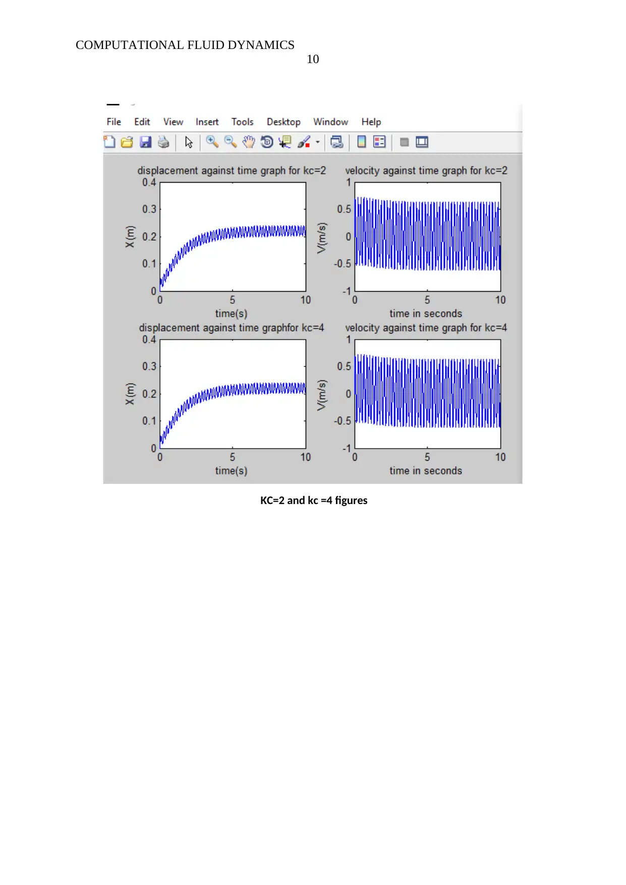
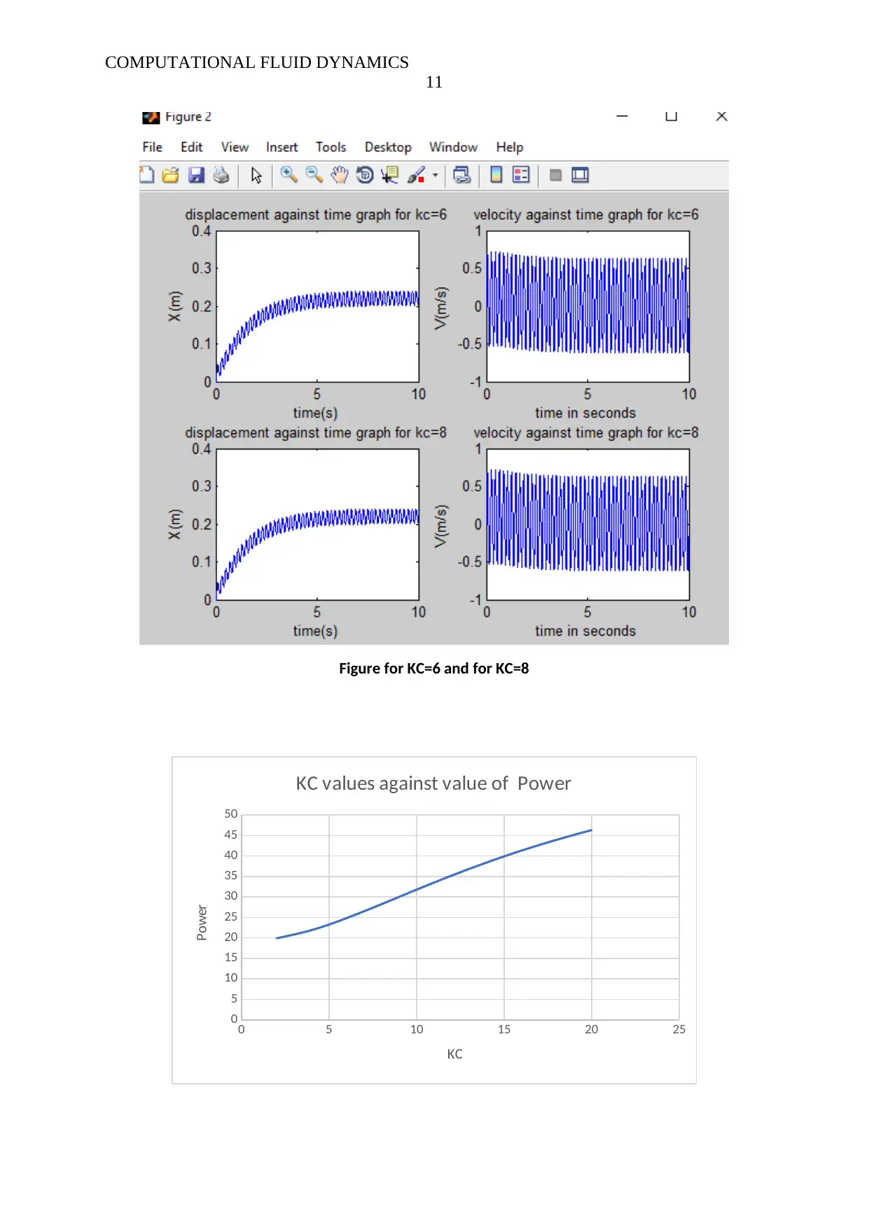
This project delves into the computational fluid dynamics (CFD) analysis of a vibrating cylinder within a fluid environment. The assignment begins with deriving the equation of motion for the cylinder, considering factors such as fluid velocity, drag force, and inertial effects. A numerical method, specifically the Fourth-order Runge-Kutta method, is then developed and implemented using MATLAB to predict the cylinder's vibration. The solution encompasses the development of a MATLAB code, which is used to simulate and analyze the cylinder's displacement, velocity, and the power generated. The results are presented in graphical formats, including displacement and velocity versus time graphs. The study further investigates the impact of varying parameters, such as the coefficient of damping and KC values, on the system's behavior. The report includes detailed explanations of the equations, numerical methods, and the interpretation of the simulation results, providing a comprehensive understanding of the cylinder vibration problem using CFD techniques. The project also discusses the 1-D convection diffusion equation and Navier-Stokes equations. Further, the project covers the stability analysis of the one-dimensional diffusion equation. The final part of the project is to study the influence of different KC and C values on the power generation.

Running HEAD: COMPUTATIONAL FLUID DYNAMICS 1
Computational fluid dynamics.
Name
Institute of affiliation
Date

COMPUTATIONAL FLUID DYNAMICS 2
KC = T Um
D
U= Water’s velocity in x direction
ρ: Water’s density
Cd: Drag force coefficient
Cm: Mass coefficient
A: = Area
Fx ( t )=D ( t )
¿ Uρ ∀ Cm+0.5 Cd AU |U |……………………….…………………………….Equation 1
velocity is defined as follows
u=U0 +sin ( 2 πt
T )Um ……………….………………………………………….. …Equation 2
U0= Steady flow velocity.
Um= flow oscillatory velocity
T= time period
Given that

COMPUTATIONAL FLUID DYNAMICS 3
P= 1
T ∫
0
T
c V 2 tⅆ ……………….…………….…………………….……………Equation 3
where P= power stored, and V is the Vibration of the system.
And
KC =U m T
D ……………….……………………………………………………..……Equation 4
It then follows that the power can be derived as follows
P=N−1
∑
n=1
N
C ( V n )
2……………….……………………………………………Equation 5
Power from the water is as follows
Fw=md CA
d V r
dt +0.5 ρ A projected CD V r∨V r∨¿……………………………………………..Equation
6
Total force Ftacting is sum of the force acting on the spring Fs, damper Fd and the water FW
Ft=FS + Fd +Fw ……………….………………………………..…………………Equation 7
Ft=−kx−c dx
dt +0.5 ρ Cd A projected|V r|V r +C A md
d2 x
d t2 ………….……………Equation 8
Since awater=¿ d2 x
d t2 equation above becomes
Ft=−kx−c dx
dt +C A md awater + 1
2 ρ Cd A p |V w−V a|(V ¿¿ w−V a )¿…………………….Equation 9
Differentiating equation 2 with respect t gives
aw=ω U m cos (ωt )……………………………………………………………………..Equation 10
awater withbe added into the f t equation¿ substitute other terms
Developing the 4th Runge kurta term
dx
dt =v………………………………………………………………………………Equation 11
dv
dt =f ( x , v )…………………………………………………………………………Equation 12

COMPUTATIONAL FLUID DYNAMICS 4
Where,
f ( x , v , t )=
kx + (c + 1
2 ρ Cd Ap |v|)v
C A md + m
………………………………………………Equation 13
x(n+ 1)∆ t =xn ∆ t + ∆ t
6 ( kx 1 +2 kx 2 +2 k x3 +k x 4 ) ………………………..Equation 14
v(n+1) ∆ t= ( kv 1 +2 kv 2 +2 kv 3 +k v 4 ) ∆t
6 + vn ∆ t …………………………Equation 15
Where,
k xa
=vn ∆ t……………………………………………………………………………Equation 16
k xb
=vn ∆ t + ∆ t
2 k v1…………………………………………………………………Equation 17
k xc
=vn ∆ t + ∆ t
2 k v2…………………………………………………………..……Equation 18
k xd
=vn ∆ t + ∆ t k v3…………………………………………………………………Equation 19
k va
=f (xn ∆ t , vn ∆ t ) …………………………………………….………………….Equation 20
k vb
=f ( xn ∆ t + ∆ t
2 k x 1 , vn ∆ t + ∆ t
2 kv 1 ) ……………………………………..…..Equation 21
k vc
=f (xn ∆ t + ∆ t
2 k x2 , vn ∆ t + ∆ t
2 kv 2) ………………..………………………Equation 22
k vd
=f (xn ∆ t + ∆ t k x 3 , vn ∆ t + ∆t kv 3 ) ………………………………………………Equation 23
In order to calculate the power from the equations above, the code below
was developed.
clear all
% Runge-Kutta method
j=7; % last digit of ID
U_m = 1+ (j/10); % Flow velocity Amplitude
U_0= 0.1 * U_m; %Velocity of steady flow
T = .2; % oscillatory flow period
D = (10+j)/100; % Diameter of cylinder
% Cylinder length
Length_cyl = 1;
mass_c = 50; % cylinder mass
rho_water = 1000; % water density

COMPUTATIONAL FLUID DYNAMICS 5
K_s = 200; % spring constant
c_d = 100; % damping coefficient
C_inertia = 1; % inertial constant
C_drag = 1.8; % Drag coefficient
om_ega = 2*pi/T; % Angular frequency of the flow
md = rho_water*pi*(D*D)/4*Length_cyl; % coefficient due to the added mass
A_projected = D*Length_cyl; % Area
delta_t = T/40; % step in time
n_delta_t = T/delta_t*50; % the total time
X_length(1:n_delta_t+1) = 0; % displacement from a step
response in time
V(1:n_delta_t+1) = 0; % velocity from a step response in
time
time(1:n_delta_t+1) = (0:n_delta_t)*delta_t;
for k=1:n_delta_t
% finding the kx1 and kv1
t_a = time(k); % defining the accelearation
a_water = om_ega*U_m*cos(om_ega*t_a); % water acceleration
V_w = U_0+U_m*sin(om_ega*t_a); % water velocity
V_a = V(k);
X_a = X_length(k);
t_1 = C_inertia*md*a_water;
t_2 = 0.5*rho_water*C_drag*A_projected*abs(V_w-V_a)*(V_w-V_a);
t_3 = -K_s*X_a-c_d*V_a;
k_x_a = V(k);
k_v_a = (t_1+t_2+t_3)/(mass_c+C_inertia*md);
% finding the k_x_b and k_v_b
t_a = time(k)+delta_t/2;
a_water = om_ega*U_m*cos(om_ega*t_a); % acceleration of the
water
V_w = U_0+U_m*sin(om_ega*t_a); % velocity of the water
V_a = V(k)+0.5*delta_t*k_v_a;
X_a = X_length(k)+0.5*delta_t*k_x_a;
t_1 = C_inertia*md*a_water;
t_2 = 0.5*rho_water*C_drag*A_projected*abs(V_w-V_a)*(V_w-V_a);
t_3 = -K_s*X_a-c_d*V_a;
k_x_b = V(k)+0.5*delta_t*k_v_a;
k_v_b = (t_1+t_2+t_3)/(mass_c+C_inertia*md);
% to calculate k_x_c and k_v_c
t_a = time(k)+delta_t/2;
a_water = om_ega*U_m*cos(om_ega*t_a); % acceleration of the
water
V_w = U_0+U_m*sin(om_ega*t_a); % velocity of the water
V_a = V(k)+0.5*delta_t*k_v_b;
X_a = X_length(k)+0.5*delta_t*k_x_b;
t_1 = C_inertia*md*a_water;
t_2 = 0.5*rho_water*C_drag*A_projected*abs(V_w-V_a)*(V_w-V_a);
t_3 = -K_s*X_a-c_d*V_a;
k_x_c = V(k)+0.5*delta_t*k_v_b;
k_v_c = (t_1+t_2+t_3)/(mass_c+C_inertia*md);
% to calculate k_x_d and
k_v_d
t_a = time(k)+delta_t;
a_water = om_ega*U_m*cos(om_ega*t_a); % acceleration of the
water
V_w = U_0+U_m*sin(om_ega*t_a); % velocity of the
water
V_a = V(k)+0.5*delta_t*k_v_c;
X_a = X_length(k)+0.5*delta_t*k_x_c;
t_1 = C_inertia*md*a_water;
t_2 = 0.5*rho_water*C_drag*A_projected*abs(V_w-V_a)*(V_w-V_a);

COMPUTATIONAL FLUID DYNAMICS 6
t_3 = -K_s*X_a-c_d*V_a;
k_x_d = V(k)+delta_t*k_v_c;
k_v_d = (t_1+t_2+t_3)/(mass_c+C_inertia*md);
% values from next step
X_length(k+1) = X_length(k)+(delta_t/6)*(k_x_a+2*k_x_b+2*k_x_c+k_x_d);
V(k+1) = V(k)+(delta_t/6)*(k_v_a+2*k_v_b+2*k_v_c+k_v_d);
end
fileID=fopen('output.txt','w');
for k= 1:n_delta_t+1
fprintf(fileID,'%12.6 %12.6 %12.6\r\n', time(k),X_length(k),V(k));
end
fclose(fileID);
%---------------------------------------------------------------------
add=0;
for m = 1:n_delta_t+1
add = add + 1/n_delta_t*c_d*(V(m)*V(m));
end
value= add;
% developing the power graph
subplot(2,2,1)
plot(time(1:n_delta_t),X_length(1:n_delta_t))
title('displacement against time graph')
xlabel('time.....(s)');
ylabel('X length.....(m)');
subplot(2,2,2);
plot(time(1:n_delta_t),V(1:n_delta_t))
xlabel('time.............seconds');
ylabel('V..............(m/s)');
title('velocity against time graph')
19.918218 is the value of the power generated

COMPUTATIONAL FLUID DYNAMICS 7
Published with MATLAB® R2018b
For constant value of C and varying value of kc
KC =U m T
D
D=0.18
T= [0.2 0.4 0.6 0.8 1.0 1.2 1.4 1.6 1.8 2.0]
Um = 1.8
Making T the subject of the formula
T = KC D
U m
Substituting the values of D, Um the formula becomes as follows
T = KC∗0.18
1.8
Below is the program to calculate the power developed from values of KC from 0 to 20
clear all
% Runge-Kutta method
j=7; % last digit of ID
U_m = 1+ (j/10); % Flow velocity Amplitude
U_0= 0.1 * U_m; %Steady flow velocity
T = .2; % oscillatory flow period
D = (10+j)/100; % cylinder diameter
% length of the cylinder
Length_cyl = 1;
mass_c = 50; % cylinder mass
rho_water = 1000; % water density
K_s = 200; % spring constant
c_d = 100; % damping coefficient
C_inertia = 1; % inertial constant
C_drag = 1.8; % coefficient of drag
om_ega = 2*pi/T; % flow`s angular frequency
md = rho_water*pi*(D*D)/4*Length_cyl; % coefficient due to the added mass
A_projected = D*Length_cyl; % projected area
delta_t = T/40; % step in time
n_delta_t = T/delta_t*50; % the total time
X_length(1:n_delta_t+1) = 0; % displacement from a step
response in time
V(1:n_delta_t+1) = 0; % velocity from a step response in
time

COMPUTATIONAL FLUID DYNAMICS 8
time(1:n_delta_t+1) = (0:n_delta_t)*delta_t;
for k=1:n_delta_t
% finding the kx1 and kv1
t_a = time(k); % defining the acceleration
a_water = om_ega*U_m*cos(om_ega*t_a); % water acceleration
V_w = U_0+U_m*sin(om_ega*t_a); % water velocity
V_a = V(k);
X_a = X_length(k);
t_1 = C_inertia*md*a_water;
t_2 = 0.5*rho_water*C_drag*A_projected*abs(V_w-V_a)*(V_w-V_a);
t_3 = -K_s*X_a-c_d*V_a;
k_x_a = V(k);
k_v_a = (t_1+t_2+t_3)/(mass_c+C_inertia*md);
% finding the k_x_b and k_v_b
t_a = time(k)+delta_t/2;
a_water = om_ega*U_m*cos(om_ega*t_a); % acceleration of the
water
V_w = U_0+U_m*sin(om_ega*t_a); % velocity of the water
V_a = V(k)+0.5*delta_t*k_v_a;
X_a = X_length(k)+0.5*delta_t*k_x_a;
t_1 = C_inertia*md*a_water;
t_2 = 0.5*rho_water*C_drag*A_projected*abs(V_w-V_a)*(V_w-V_a);
t_3 = -K_s*X_a-c_d*V_a;
k_x_b = V(k)+0.5*delta_t*k_v_a;
k_v_b = (t_1+t_2+t_3)/(mass_c+C_inertia*md);
% to calculate k_x_c and k_v_c
t_a = time(k)+delta_t/2;
a_water = om_ega*U_m*cos(om_ega*t_a); % acceleration of the
water
V_w = U_0+U_m*sin(om_ega*t_a); % velocity of the water
V_a = V(k)+0.5*delta_t*k_v_b;
X_a = X_length(k)+0.5*delta_t*k_x_b;
t_1 = C_inertia*md*a_water;
t_2 = 0.5*rho_water*C_drag*A_projected*abs(V_w-V_a)*(V_w-V_a);
t_3 = -K_s*X_a-c_d*V_a;
k_x_c = V(k)+0.5*delta_t*k_v_b;
k_v_c = (t_1+t_2+t_3)/(mass_c+C_inertia*md);
% to calculate k_x_d and
k_v_d
t_a = time(k)+delta_t;
a_water = om_ega*U_m*cos(om_ega*t_a); % acceleration of the
water
V_w = U_0+U_m*sin(om_ega*t_a); % velocity of the
water
V_a = V(k)+0.5*delta_t*k_v_c;
X_a = X_length(k)+0.5*delta_t*k_x_c;
t_1 = C_inertia*md*a_water;
t_2 = 0.5*rho_water*C_drag*A_projected*abs(V_w-V_a)*(V_w-V_a);
t_3 = -K_s*X_a-c_d*V_a;
k_x_d = V(k)+delta_t*k_v_c;
k_v_d = (t_1+t_2+t_3)/(mass_c+C_inertia*md);
% values from next step
X_length(k+1) = X_length(k)+(delta_t/6)*(k_x_a+2*k_x_b+2*k_x_c+k_x_d);
V(k+1) = V(k)+(delta_t/6)*(k_v_a+2*k_v_b+2*k_v_c+k_v_d);
end
fileID=fopen('output.txt','w');
for k= 1:n_delta_t+1
fprintf(fileID,'%12.6 %12.6 %12.6\r\n', time(k),X_length(k),V(k));
end
fclose(fileID);

COMPUTATIONAL FLUID DYNAMICS 9
%---------------------------------------------------------------------
add=0;
for m = 1:n_delta_t+1
add = add + 1/n_delta_t*c_d*(V(m)*V(m));
end
value= add;
% developing the power graph
subplot(2,2,1)
plot(time(1:n_delta_t),X_length(1:n_delta_t))
title('displacement against time graph')
xlabel('time.....(s)');
ylabel('X length.....(m)');
subplot(2,2,2);
plot(time(1:n_delta_t),V(1:n_delta_t))
xlabel('time.............seconds');
ylabel('V..............(m/s)');
title('velocity against time graph')
24.832199 is the value of power generated
Published with MATLAB® R2014b
The table below gives the power generated for Different values of KC is given in table below:
KC T P
2.00 0.200 19.9
4.00 0.400 21.9
6.00 0.600 24.8
8.00 0.800 28.2
10.00 1.000 31.8
12.00 1.200 35.2
14.00 1.400 38.4
16.00 1.600 41.3
18.00 1.800 43.9
20.00 2.000 46.3

COMPUTATIONAL FLUID DYNAMICS
10
KC=2 and kc =4 figures

COMPUTATIONAL FLUID DYNAMICS
11
Figure for KC=6 and for KC=8
0 5 10 15 20 25
0
5
10
15
20
25
30
35
40
45
50
KC values against value of Power
KC
Power

COMPUTATIONAL FLUID DYNAMICS
12
The graph above shows power increases gradually from 19.91822 to 46.31243.
 Holding KC constant at a value of 10, and conducting simulations for c=0 to 2000 N·m/s with at
an interval of 50 power variation becomes as in the table below
KC T P
2.00 0.200 19.9
4.00 0.400 21.9
6.00 0.600 24.8
8.00 0.800 28.2
10.00 1.000 31.8
12.00 1.200 35.2
14.00 1.400 38.4
16.00 1.600 41.3
18.00 1.800 43.9
20.00 2.000 46.3
Power for given k values
c power
0.0 0.0
50.0 17.4
100.0 31.8
150.0 43.4
200.0 52.7
250.0 59.9
300.0 65.4
350.0 69.4
400.0 72.2
450.0 74.2
500.0 75.4
550.0 76.0
600.0 76.2
650.0 76.1
700.0 75.7
750.0 75.1
800.0 74.3
850.0 73.5
900.0 72.5
950.0 71.5
1000.0 70.5
1050.0 69.4