Computational Problem Solving: Basic Statistics, Sets, and Python
VerifiedAdded on 2023/01/13
|34
|11357
|29
Lecture Notes
AI Summary
These lecture notes provide a comprehensive introduction to computational problem solving using Python, focusing on fundamental statistical concepts and data structures. The content covers descriptive statistics, including measures of central tendency (arithmetic, geometric, and harmonic means), data types, sampling methods, and the misuse of statistics. It also delves into the basics of data structures such as linked lists, queues, rings, sets, and dictionaries in Python, along with string and file manipulation techniques. The notes include mathematical and programming questions to reinforce understanding and application of the concepts. The lecture also touches upon the application of statistics and programming in the field of data science, illustrating the power of data analysis with real-world examples, such as Netflix recommendation algorithms and targeted advertising. This resource, available on Desklib, aims to equip students with the foundational knowledge and practical skills needed for data analysis and programming in Python.
Lecture Notes
Computational Problem Solving
Week 5:
Basic Statistics, Sets and Tuples, Dictionaries
and String / File Manipulation in Python
Contents:
Contents
Basic Statistics ............................................................................................................................................................... 2
Types of Data and Sampling ......................................................................................................................................... 2
Arithmetic Mean, Geometric Mean and Harmonic Mean ........................................................................................... 4
Median and Mode ........................................................................................................................................................ 8
Interquartile Range and Standard Deviation ................................................................................................................ 9
Parametric and Non-parametric Data ........................................................................................................................ 13
Regression and Correlation ........................................................................................................................................ 14
Misuse of Statistics ..................................................................................................................................................... 16
Introduction to Data Structures ................................................................................................................................. 18
Linked Lists .............................................................................................................................................................. 18
Queues .................................................................................................................................................................... 19
Rings ....................................................................................................................................................................... 23
Sets in Python ............................................................................................................................................................. 24
Dictionaries ................................................................................................................................................................. 27
Error Handling ................................................................................................................ Error! Bookmark not defined.
String Manipulation .................................................................................................................................................... 29
File Manipulation ........................................................................................................................................................ 31
Mathematics Questions .............................................................................................................................................. 32
Programming Questions ............................................................................................................................................. 33
Paraphrase This Document
Need a fresh take? Get an instant paraphrase of this document with our AI Paraphraser
Basic Statistics
Descriptive statistics is the process of summarising data. You would have looked at some aspects of this from
school. Another area of statistics is called inference which is inferring something from the data given (which leads
to prediction). The combination of statistics and programming is often referred to as data analysis and data
science. Data science is one of the hottest areas of computer science currently and is used throughout the
modern world. For example, when you think about what to watch next on Netflix, the internal algorithms will
predict possible shows to watch based on your previous viewing habits. Likewise, when you purchase items from
amazon. One of the main tools used for data science is Python together with some libraries to make it both easier
and more efficient. Another popular programming tool for statistics is R.
One infamous story about the power of data science is the following:
Meeting with a Target manager while clutching some printed ads that had been delivered to his home, a
customer was outraged by their product placement aimed at his young daughter. 'My daughter got this in the
mail!' the man said to the manager according to the Times, showing him the store's coupons advertising baby-
related products. 'She's still in high school, and you're sending her coupons for baby clothes and cribs? Are you
trying to encourage her to get pregnant?' the man asked the manager who responded with a baffled apology. The
manager himself didn't know why the man's daughter had received the items. He followed up with a phone call to
him later on, apologizing again. What the manager didn't know was that the company's analytics department
most likely had noticed a pattern of products related to early pregnancy purchased by the man's daughter. Clues
such as vitamin supplements, large quantities of lotion, and hand sanitizers, typical to many pregnant women
according to the Target department, signal other items the consumer may need. Or as a woman's pregnancy
continues, what she will soon need, like nappys. 'I had a talk with my daughter,' the man responded later to the
Target manager after listening to his second apology on the phone. 'It turns out there's been some activities in my
house I haven't been completely aware of. She's due in August. I owe you an apology,' he said.
So, when you use your clubcard, Tescos are monitoring your data to see what you might want to buy to target
vouchers to your potential spending habits.
Types of Data and Sampling
Data is often categorised into qualitative and quantitative. Qualitative data is data which is not numerical. For
example, favourite colours would be a type of qualitative data. Conversely, quantitative data is data that is
numerical, for example shoe size, height, etc.
Quantitative data itself may also be split into two categories to make analysis easier. These two partitions are
discrete data and continuous data.
Discrete data is data such as shoe size which are distinct values, e.g. 6, 6.5, 7, 7.5. You are unable to by a size 7.12
shoe, for example. On the other hand, continuous data has no such distinct values. For example, the height of a
person may be 1.62m but if we had a better way to measure it, we might find the height is actually 1.617m, and
we might be able to measure the height even more precisely. Sometimes, it can be convenient to discretise data
to make it easier to analyse or put data into “bins”. For example, for height, as we cannot measure the exact
height of a person, we might put it into a category of, say, 160𝑐𝑚 ≤ ℎ < 165𝑐𝑚with some other bins, such as
165𝑐𝑚 ≤ ℎ > 170𝑐𝑚. It is important that when we are placing data into these bins that there are no overlaps
between the categories.
Definition 9.1
A population is the set of things that you are interested in.
A sample is a subset of the population
The population may be finite, such as the films currently in the cinema or infinite, such as the possible locations
that an archers arrow might land in. Parameters for a population can be almost impossible to accurately measure,
so it is best to take a statistic from a sample and use that result to say something about the population.
Definition 9.2
A parameter is a number that describes the entire population. A statistic is a number taken from a
single sample— you can use one or more of these to estimate the parameter.
The population might be large, say the population of the UK, and any statistics would be hard to gather. A census
is when data is collected from the whole population of interest. In terms of the UK, there is a census every ten
years to collect data about the population to help ascertain where to place money for large infrastructure
projects (amongst other uses).
A sample, as previously mentioned, is a subset of the population. There are many different techniques to gather a
sample and these depend on the situation and intended use of the data.
Sampling Method Description
Sample random
sampling
Every member of the population is equally likely to be chosen. For example,
allocate each member of the population a number. Then use random
numbers to choose a sample of the desired size.
Systematic sampling Find a sample of size 𝑛 from a population of size 𝑁by taking one member
from the first 𝑘 members of the population at random and then selecting
every 𝑘𝑡ℎmember after that, where 𝑘 = 𝑁
𝑛
Stratified sampling When you know you want distinct groups to be represented in your sample,
split the population into these distinct groups and then sample within each
group in proportion to its size.
Opportunity sampling Take samples from members of the population you have access to until you
have a sample of the desired size.
Quota sampling When you know you want distinct groups to be represented in your sample,
decide how many members of each group you wish to sample in advance
and use opportunity sampling until you have a large enough sample for
each group.
Cluster sampling Split the population into clusters that you expect to be similar to each
other, then take a sample from each of these clusters.
Within these broad categories, further refinements might be made, e.g., to choose the sample within the
stratified sampling or combined with other methods (e.g., a combination of stratified sampling and then
opportunity sampling). Often the sampling method is constrained by the data collection. Systematic sampling can
only be used if we can list the data and assign a identifier with each item. Sometimes due to ethical reasons (e.g.,
drug testing) have to use opportunity sampling as you cannot just ask random people on the street.
Sometimes there is bias within the sampling method. A bias is a flaw in the sampling procedure that makes it
more likely that the sample will not be representative of the population. Examples of where bias occurs is: faulty
sampling (sample is not representative), leading questions (questions are worded as to influence the answers),
faulty interviewing (failure to interview the entire sample, misreading questions, misinterpreting what was said),
lack of knowledge or understanding (person being interviewed does not understand or does not have the
information needed) and false answers (person being interviewed intentionally gives incorrect information).
There are some famous examples of bias within sampling, for example, during the Brexit referendum where the
remain campaign was thought to have won due to interviewers asking only select populations and people lying
due to peer pressure (this has also happened in various general elections).
⊘ This is a preview!⊘
Do you want full access?
Subscribe today to unlock all pages.
Trusted by 1+ million students worldwide
Arithmetic Mean, Geometric Mean and Harmonic Mean
The arithmetic mean is the most common type of average. All averages are called a measure of central tendency
and is a metric to summarise a typical data value. The choice of average is very much dependent on both the
application and the type of data being analysed.
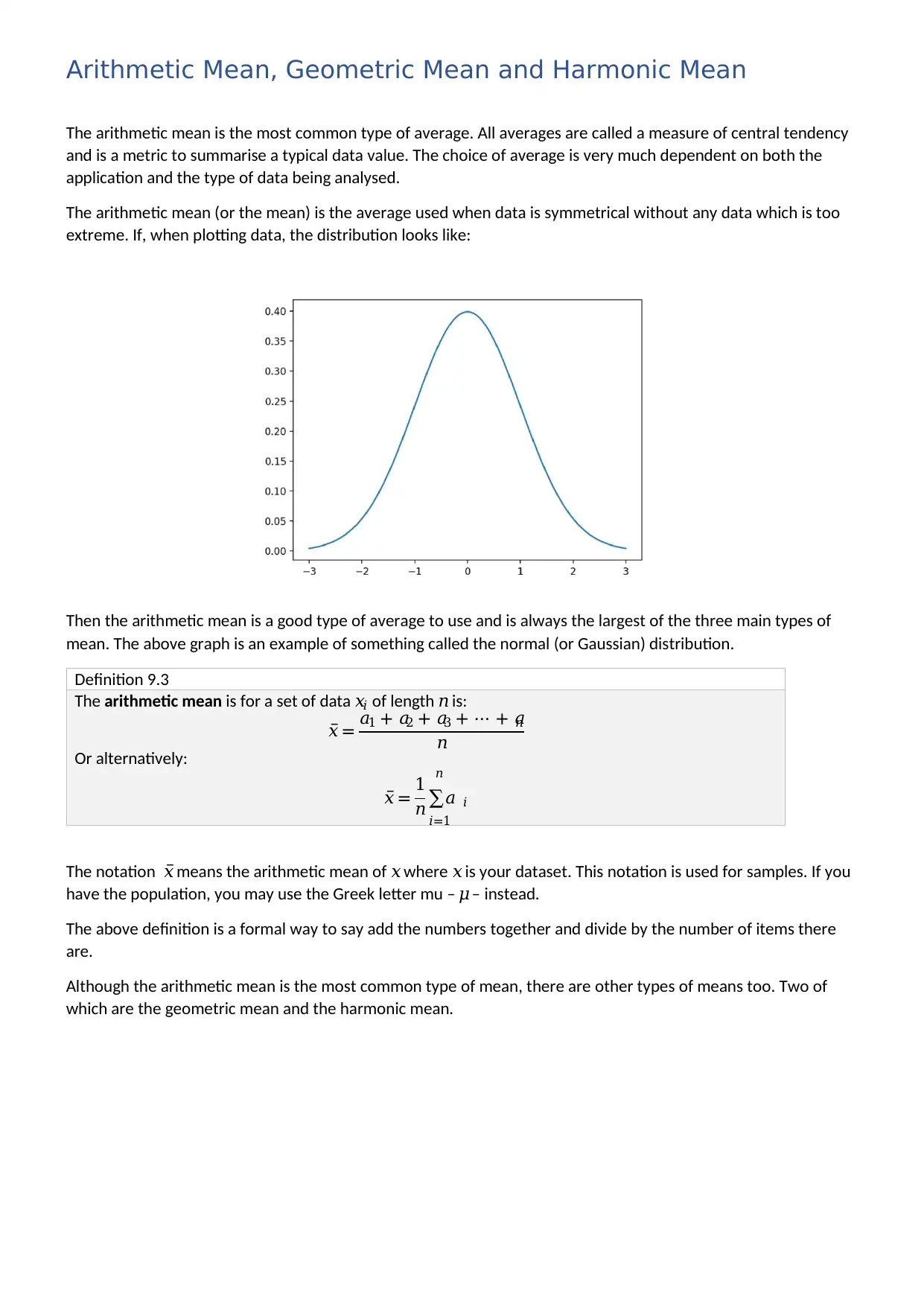
The arithmetic mean (or the mean) is the average used when data is symmetrical without any data which is too
extreme. If, when plotting data, the distribution looks like:
Then the arithmetic mean is a good type of average to use and is always the largest of the three main types of
mean. The above graph is an example of something called the normal (or Gaussian) distribution.
Definition 9.3
The arithmetic mean is for a set of data 𝑥𝑖 of length 𝑛 is:
𝑥̅ = 𝑎1 + 𝑎2 + 𝑎3 + ⋯ + 𝑎𝑛
𝑛
Or alternatively:
𝑥̅ = 1
𝑛∑𝑎 𝑖
𝑛
𝑖=1
The notation 𝑥̅ means the arithmetic mean of 𝑥 where 𝑥 is your dataset. This notation is used for samples. If you
have the population, you may use the Greek letter mu – 𝜇 – instead.
The above definition is a formal way to say add the numbers together and divide by the number of items there
are.
Although the arithmetic mean is the most common type of mean, there are other types of means too. Two of
which are the geometric mean and the harmonic mean.
The arithmetic mean is the most common type of average. All averages are called a measure of central tendency
and is a metric to summarise a typical data value. The choice of average is very much dependent on both the
application and the type of data being analysed.
The arithmetic mean (or the mean) is the average used when data is symmetrical without any data which is too
extreme. If, when plotting data, the distribution looks like:
Then the arithmetic mean is a good type of average to use and is always the largest of the three main types of
mean. The above graph is an example of something called the normal (or Gaussian) distribution.
Definition 9.3
The arithmetic mean is for a set of data 𝑥𝑖 of length 𝑛 is:
𝑥̅ = 𝑎1 + 𝑎2 + 𝑎3 + ⋯ + 𝑎𝑛
𝑛
Or alternatively:
𝑥̅ = 1
𝑛∑𝑎 𝑖
𝑛
𝑖=1
The notation 𝑥̅ means the arithmetic mean of 𝑥 where 𝑥 is your dataset. This notation is used for samples. If you
have the population, you may use the Greek letter mu – 𝜇 – instead.
The above definition is a formal way to say add the numbers together and divide by the number of items there
are.
Although the arithmetic mean is the most common type of mean, there are other types of means too. Two of
which are the geometric mean and the harmonic mean.
Paraphrase This Document
Need a fresh take? Get an instant paraphrase of this document with our AI Paraphraser
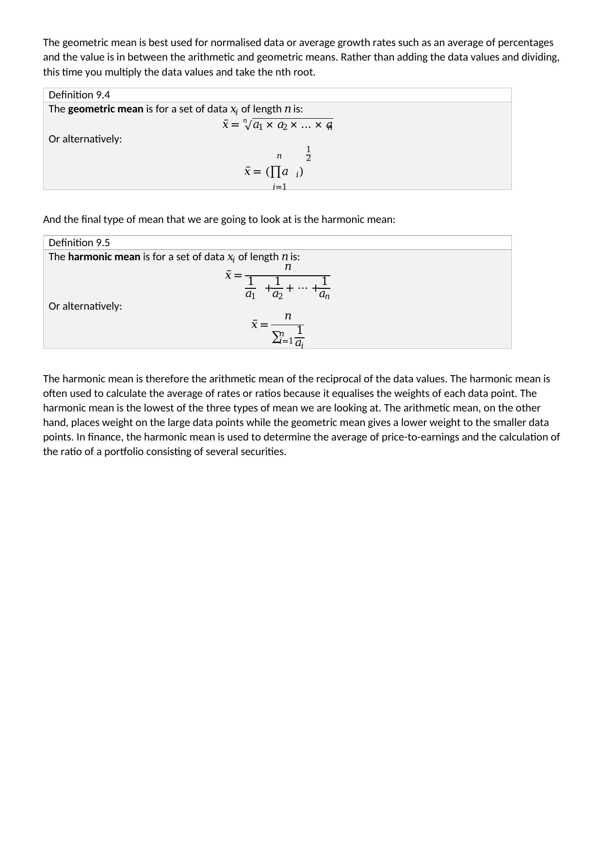
The geometric mean is best used for normalised data or average growth rates such as an average of percentages
and the value is in between the arithmetic and geometric means. Rather than adding the data values and dividing,
this time you multiply the data values and take the nth root.
Definition 9.4
The geometric mean is for a set of data 𝑥𝑖 of length 𝑛 is:
𝑥̅ = √𝑎1 × 𝑎2 × … × 𝑎𝑛
𝑛
Or alternatively:
𝑥̅ = (∏𝑎 𝑖
𝑛
𝑖=1
)
1
2
And the final type of mean that we are going to look at is the harmonic mean:
Definition 9.5
The harmonic mean is for a set of data 𝑥𝑖 of length 𝑛 is:
𝑥̅ = 𝑛
1
𝑎1 + 1
𝑎2 + ⋯ +1
𝑎𝑛
Or alternatively:
𝑥̅ = 𝑛
∑ 1
𝑎𝑖
𝑛
𝑖=1
The harmonic mean is therefore the arithmetic mean of the reciprocal of the data values. The harmonic mean is
often used to calculate the average of rates or ratios because it equalises the weights of each data point. The
harmonic mean is the lowest of the three types of mean we are looking at. The arithmetic mean, on the other
hand, places weight on the large data points while the geometric mean gives a lower weight to the smaller data
points. In finance, the harmonic mean is used to determine the average of price-to-earnings and the calculation of
the ratio of a portfolio consisting of several securities.
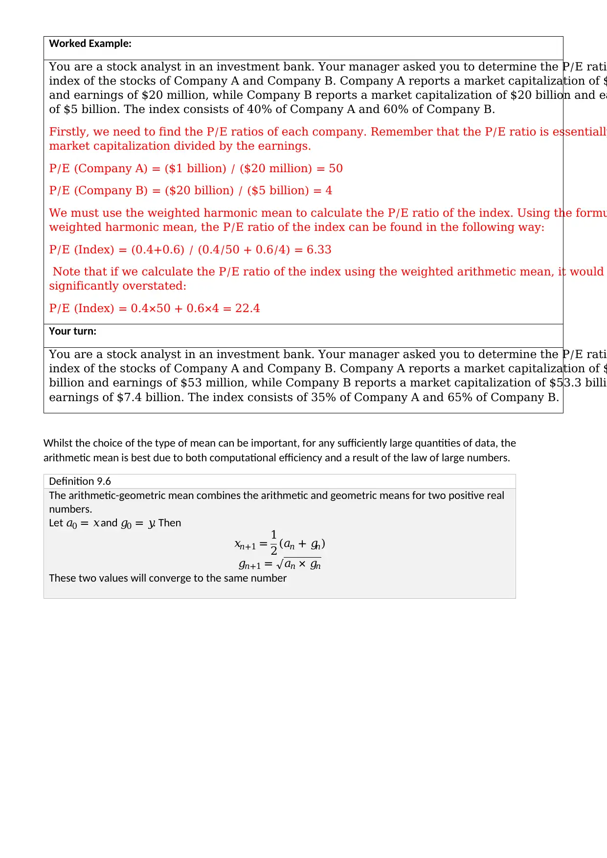
Worked Example:
You are a stock analyst in an investment bank. Your manager asked you to determine the P/E rati
index of the stocks of Company A and Company B. Company A reports a market capitalization of $
and earnings of $20 million, while Company B reports a market capitalization of $20 billion and ea
of $5 billion. The index consists of 40% of Company A and 60% of Company B.
Firstly, we need to find the P/E ratios of each company. Remember that the P/E ratio is essentially
market capitalization divided by the earnings.
P/E (Company A) = ($1 billion) / ($20 million) = 50
P/E (Company B) = ($20 billion) / ($5 billion) = 4
We must use the weighted harmonic mean to calculate the P/E ratio of the index. Using the formu
weighted harmonic mean, the P/E ratio of the index can be found in the following way:
P/E (Index) = (0.4+0.6) / (0.4/50 + 0.6/4) = 6.33
Note that if we calculate the P/E ratio of the index using the weighted arithmetic mean, it would
significantly overstated:
P/E (Index) = 0.4×50 + 0.6×4 = 22.4
Your turn:
You are a stock analyst in an investment bank. Your manager asked you to determine the P/E rati
index of the stocks of Company A and Company B. Company A reports a market capitalization of $
billion and earnings of $53 million, while Company B reports a market capitalization of $53.3 billi
earnings of $7.4 billion. The index consists of 35% of Company A and 65% of Company B.
Whilst the choice of the type of mean can be important, for any sufficiently large quantities of data, the
arithmetic mean is best due to both computational efficiency and a result of the law of large numbers.
Definition 9.6
The arithmetic-geometric mean combines the arithmetic and geometric means for two positive real
numbers.
Let 𝑎0 = 𝑥and 𝑔0 = 𝑦. Then
𝑥𝑛+1 = 1
2(𝑎𝑛 + 𝑔𝑛)
𝑔𝑛+1 = √𝑎𝑛 × 𝑔𝑛
These two values will converge to the same number
You are a stock analyst in an investment bank. Your manager asked you to determine the P/E rati
index of the stocks of Company A and Company B. Company A reports a market capitalization of $
and earnings of $20 million, while Company B reports a market capitalization of $20 billion and ea
of $5 billion. The index consists of 40% of Company A and 60% of Company B.
Firstly, we need to find the P/E ratios of each company. Remember that the P/E ratio is essentially
market capitalization divided by the earnings.
P/E (Company A) = ($1 billion) / ($20 million) = 50
P/E (Company B) = ($20 billion) / ($5 billion) = 4
We must use the weighted harmonic mean to calculate the P/E ratio of the index. Using the formu
weighted harmonic mean, the P/E ratio of the index can be found in the following way:
P/E (Index) = (0.4+0.6) / (0.4/50 + 0.6/4) = 6.33
Note that if we calculate the P/E ratio of the index using the weighted arithmetic mean, it would
significantly overstated:
P/E (Index) = 0.4×50 + 0.6×4 = 22.4
Your turn:
You are a stock analyst in an investment bank. Your manager asked you to determine the P/E rati
index of the stocks of Company A and Company B. Company A reports a market capitalization of $
billion and earnings of $53 million, while Company B reports a market capitalization of $53.3 billi
earnings of $7.4 billion. The index consists of 35% of Company A and 65% of Company B.
Whilst the choice of the type of mean can be important, for any sufficiently large quantities of data, the
arithmetic mean is best due to both computational efficiency and a result of the law of large numbers.
Definition 9.6
The arithmetic-geometric mean combines the arithmetic and geometric means for two positive real
numbers.
Let 𝑎0 = 𝑥and 𝑔0 = 𝑦. Then
𝑥𝑛+1 = 1
2(𝑎𝑛 + 𝑔𝑛)
𝑔𝑛+1 = √𝑎𝑛 × 𝑔𝑛
These two values will converge to the same number
⊘ This is a preview!⊘
Do you want full access?
Subscribe today to unlock all pages.
Trusted by 1+ million students worldwide
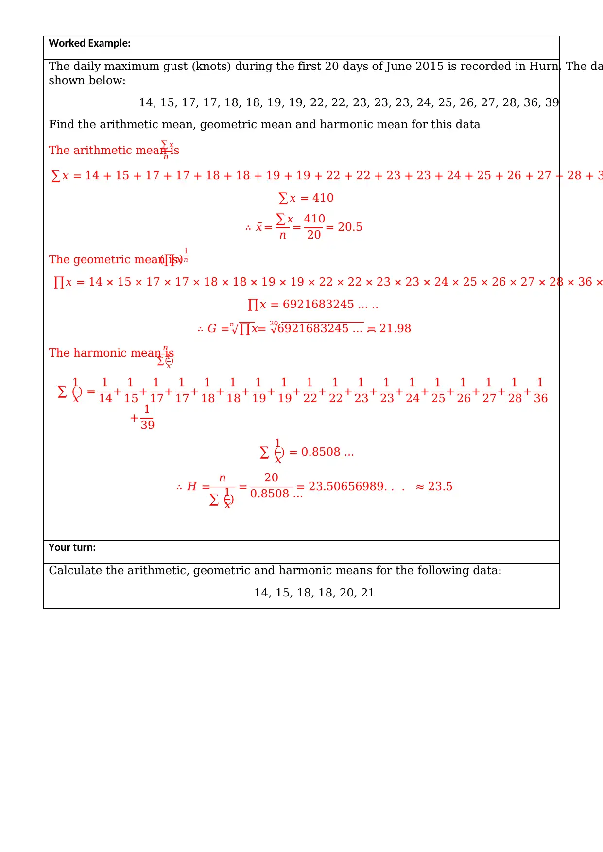
Worked Example:
The daily maximum gust (knots) during the first 20 days of June 2015 is recorded in Hurn. The da
shown below:
14, 15, 17, 17, 18, 18, 19, 19, 22, 22, 23, 23, 23, 24, 25, 26, 27, 28, 36, 39
Find the arithmetic mean, geometric mean and harmonic mean for this data
The arithmetic mean is
∑𝑥
𝑛
∑𝑥 = 14 + 15 + 17 + 17 + 18 + 18 + 19 + 19 + 22 + 22 + 23 + 23 + 24 + 25 + 26 + 27 + 28 + 3
∑𝑥 = 410
∴ 𝑥̅= ∑𝑥
𝑛 = 410
20 = 20.5
The geometric mean is(∏𝑥)1
𝑛
∏𝑥 = 14 × 15 × 17 × 17 × 18 × 18 × 19 × 19 × 22 × 22 × 23 × 23 × 24 × 25 × 26 × 27 × 28 × 36 ×
∏𝑥 = 6921683245 … ..
∴ 𝐺 = √∏𝑥𝑛 = √6921683245 … . .
20
= 21.98
The harmonic mean is
𝑛
∑(1
𝑥)
∑ (
1
𝑥) = 1
14+ 1
15+ 1
17+ 1
17+ 1
18+ 1
18+ 1
19+ 1
19+ 1
22+ 1
22+ 1
23+ 1
23+ 1
24+ 1
25+ 1
26+ 1
27+ 1
28+ 1
36
+ 1
39
∑ (
1
𝑥) = 0.8508 …
∴ 𝐻 = 𝑛
∑ (
1
𝑥)
= 20
0.8508 …
= 23.50656989. . . ≈ 23.5
Your turn:
Calculate the arithmetic, geometric and harmonic means for the following data:
14, 15, 18, 18, 20, 21
Paraphrase This Document
Need a fresh take? Get an instant paraphrase of this document with our AI Paraphraser
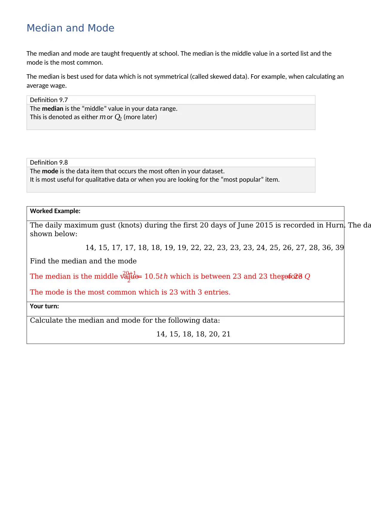
Median and Mode
The median and mode are taught frequently at school. The median is the middle value in a sorted list and the
mode is the most common.
The median is best used for data which is not symmetrical (called skewed data). For example, when calculating an
average wage.
Definition 9.7
The median is the “middle” value in your data range.
This is denoted as either 𝑚 or 𝑄2 (more later)
Definition 9.8
The mode is the data item that occurs the most often in your dataset.
It is most useful for qualitative data or when you are looking for the “most popular” item.
Worked Example:
The daily maximum gust (knots) during the first 20 days of June 2015 is recorded in Hurn. The da
shown below:
14, 15, 17, 17, 18, 18, 19, 19, 22, 22, 23, 23, 23, 24, 25, 26, 27, 28, 36, 39
Find the median and the mode
The median is the middle value
20+1
2 = 10.5𝑡ℎ which is between 23 and 23 therefore 𝑄2 = 23
The mode is the most common which is 23 with 3 entries.
Your turn:
Calculate the median and mode for the following data:
14, 15, 18, 18, 20, 21
Interquartile Range and Standard Deviation
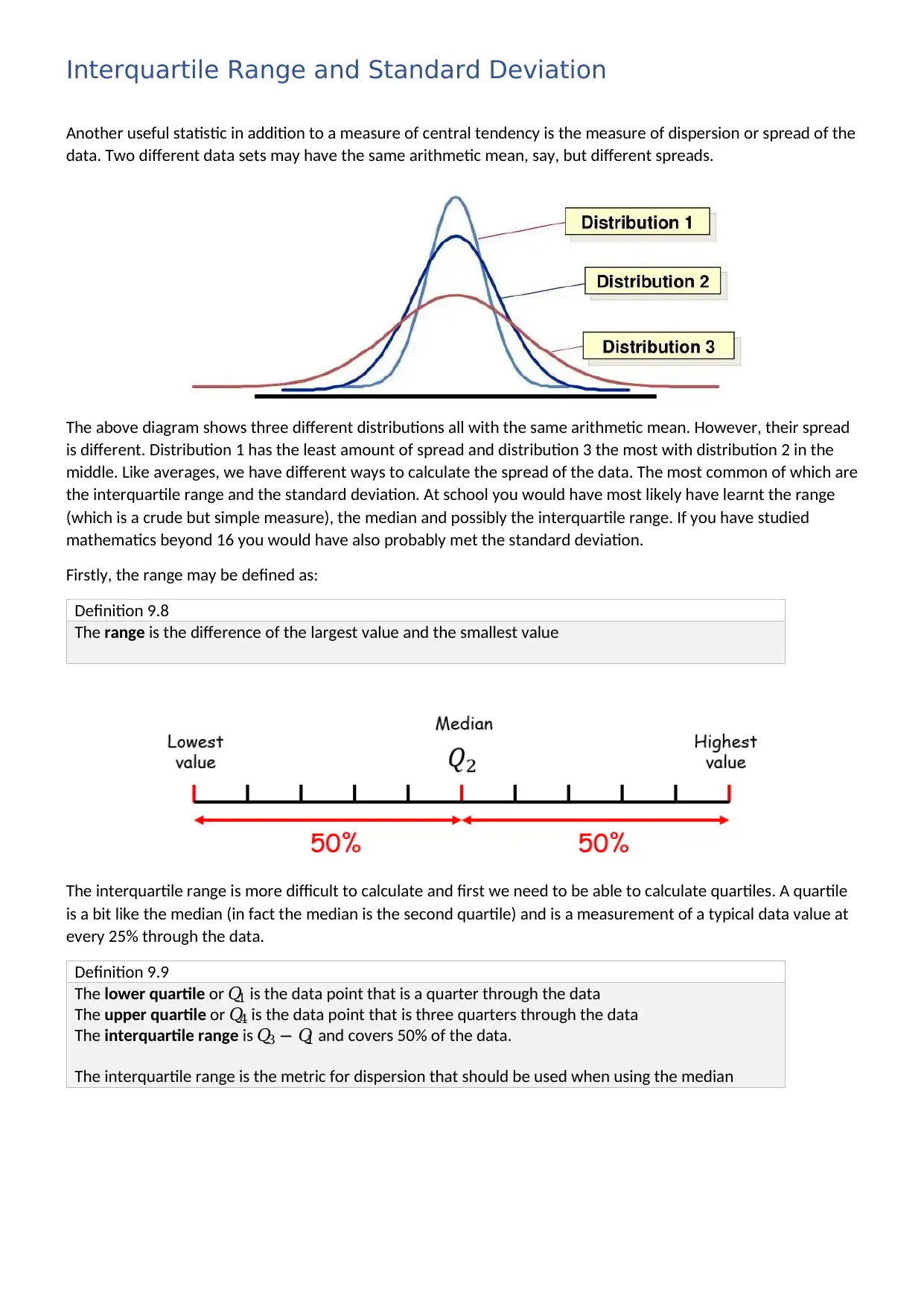
Another useful statistic in addition to a measure of central tendency is the measure of dispersion or spread of the
data. Two different data sets may have the same arithmetic mean, say, but different spreads.
The above diagram shows three different distributions all with the same arithmetic mean. However, their spread
is different. Distribution 1 has the least amount of spread and distribution 3 the most with distribution 2 in the
middle. Like averages, we have different ways to calculate the spread of the data. The most common of which are
the interquartile range and the standard deviation. At school you would have most likely have learnt the range
(which is a crude but simple measure), the median and possibly the interquartile range. If you have studied
mathematics beyond 16 you would have also probably met the standard deviation.
Firstly, the range may be defined as:
Definition 9.8
The range is the difference of the largest value and the smallest value
The interquartile range is more difficult to calculate and first we need to be able to calculate quartiles. A quartile
is a bit like the median (in fact the median is the second quartile) and is a measurement of a typical data value at
every 25% through the data.
Definition 9.9
The lower quartile or 𝑄1 is the data point that is a quarter through the data
The upper quartile or 𝑄4 is the data point that is three quarters through the data
The interquartile range is 𝑄3 − 𝑄1 and covers 50% of the data.
The interquartile range is the metric for dispersion that should be used when using the median
⊘ This is a preview!⊘
Do you want full access?
Subscribe today to unlock all pages.
Trusted by 1+ million students worldwide
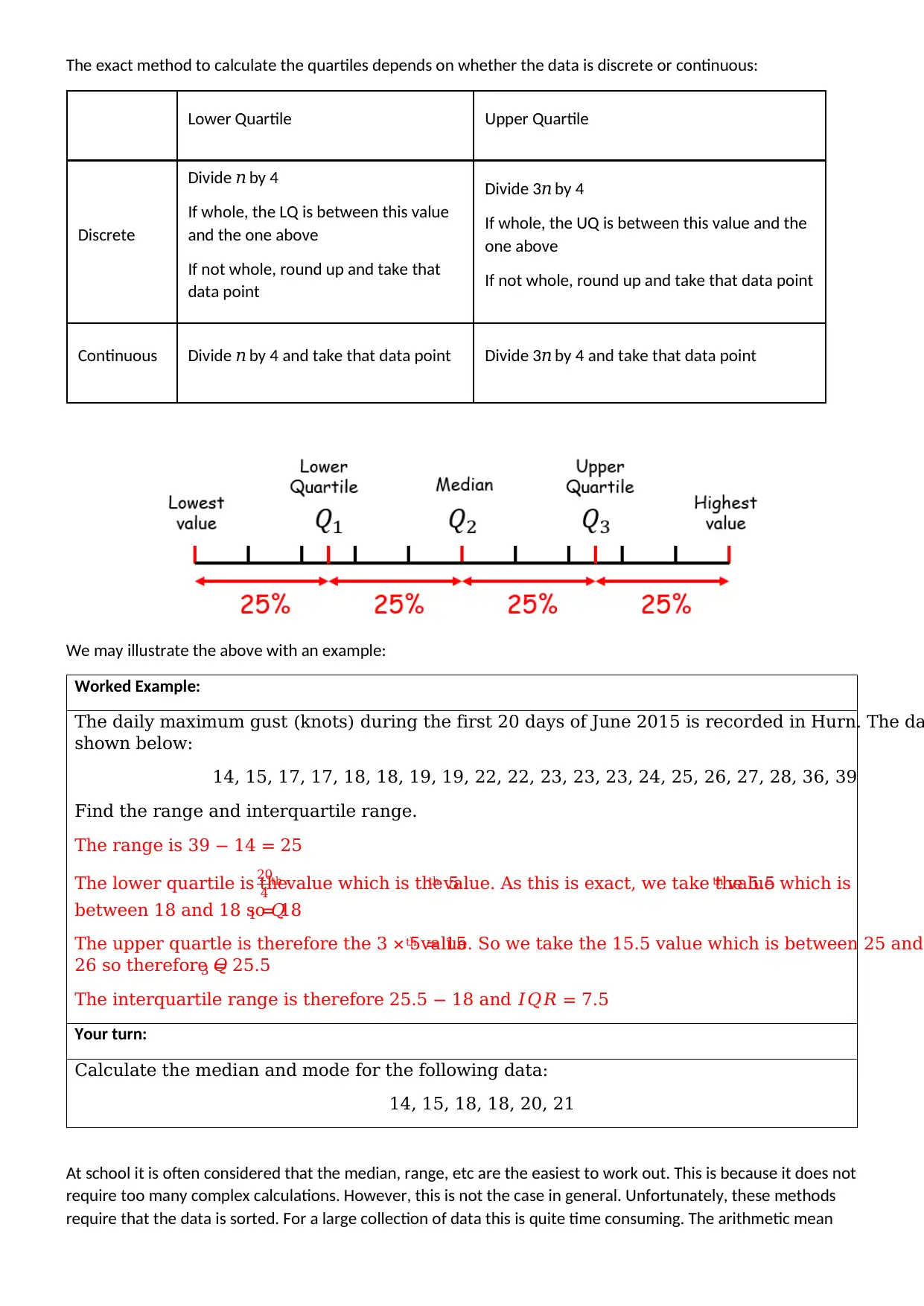
The exact method to calculate the quartiles depends on whether the data is discrete or continuous:
Lower Quartile Upper Quartile
Discrete
Divide 𝑛 by 4
If whole, the LQ is between this value
and the one above
If not whole, round up and take that
data point
Divide 3𝑛 by 4
If whole, the UQ is between this value and the
one above
If not whole, round up and take that data point
Continuous Divide 𝑛 by 4 and take that data point Divide 3𝑛 by 4 and take that data point
We may illustrate the above with an example:
Worked Example:
The daily maximum gust (knots) during the first 20 days of June 2015 is recorded in Hurn. The da
shown below:
14, 15, 17, 17, 18, 18, 19, 19, 22, 22, 23, 23, 23, 24, 25, 26, 27, 28, 36, 39
Find the range and interquartile range.
The range is 39 − 14 = 25
The lower quartile is the
20
4 th value which is the 5th value. As this is exact, we take the 5.5th value which is
between 18 and 18 so 𝑄1 = 18
The upper quartle is therefore the 3 × 5 = 15th value. So we take the 15.5 value which is between 25 and
26 so therefore 𝑄3 = 25.5
The interquartile range is therefore 25.5 − 18 and 𝐼𝑄𝑅 = 7.5
Your turn:
Calculate the median and mode for the following data:
14, 15, 18, 18, 20, 21
At school it is often considered that the median, range, etc are the easiest to work out. This is because it does not
require too many complex calculations. However, this is not the case in general. Unfortunately, these methods
require that the data is sorted. For a large collection of data this is quite time consuming. The arithmetic mean
Paraphrase This Document
Need a fresh take? Get an instant paraphrase of this document with our AI Paraphraser
and standard deviation rely mostly on addition and so is more efficient for larger datasets. Luckily, the central
limit theorem and the law of large numbers can be used to approximate any distribution as a symmetric (normal)
distribution given enough data.
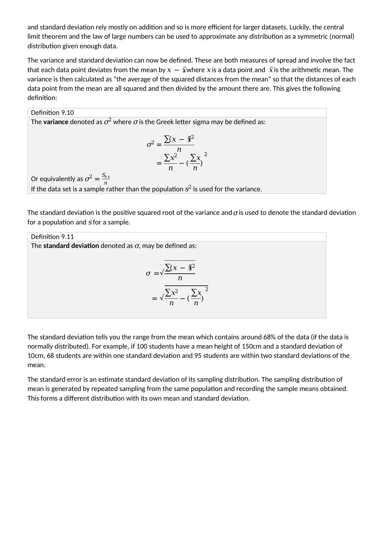
The variance and standard deviation can now be defined. These are both measures of spread and involve the fact
that each data point deviates from the mean by 𝑥 − 𝑥̅, where 𝑥 is a data point and 𝑥̅ is the arithmetic mean. The
variance is then calculated as “the average of the squared distances from the mean” so that the distances of each
data point from the mean are all squared and then divided by the amount there are. This gives the following
definition:
Definition 9.10
The variance denoted as 𝜎2 where 𝜎is the Greek letter sigma may be defined as:
𝜎2 = ∑(𝑥 − 𝑥̅)2
𝑛
= ∑𝑥2
𝑛 − ( ∑𝑥
𝑛 )
2
Or equivalently as 𝜎2 = 𝑆𝑥𝑥
𝑛
If the data set is a sample rather than the population 𝑠2 is used for the variance.
The standard deviation is the positive squared root of the variance and 𝜎is used to denote the standard deviation
for a population and 𝑠 for a sample.
Definition 9.11
The standard deviation denoted as 𝜎, may be defined as:
𝜎 =√∑(𝑥 − 𝑥̅)2
𝑛
= √∑𝑥2
𝑛 − ( ∑𝑥
𝑛 )
2
The standard deviation tells you the range from the mean which contains around 68% of the data (if the data is
normally distributed). For example, if 100 students have a mean height of 150cm and a standard deviation of
10cm, 68 students are within one standard deviation and 95 students are within two standard deviations of the
mean.
The standard error is an estimate standard deviation of its sampling distribution. The sampling distribution of
mean is generated by repeated sampling from the same population and recording the sample means obtained.
This forms a different distribution with its own mean and standard deviation.
limit theorem and the law of large numbers can be used to approximate any distribution as a symmetric (normal)
distribution given enough data.
The variance and standard deviation can now be defined. These are both measures of spread and involve the fact
that each data point deviates from the mean by 𝑥 − 𝑥̅, where 𝑥 is a data point and 𝑥̅ is the arithmetic mean. The
variance is then calculated as “the average of the squared distances from the mean” so that the distances of each
data point from the mean are all squared and then divided by the amount there are. This gives the following
definition:
Definition 9.10
The variance denoted as 𝜎2 where 𝜎is the Greek letter sigma may be defined as:
𝜎2 = ∑(𝑥 − 𝑥̅)2
𝑛
= ∑𝑥2
𝑛 − ( ∑𝑥
𝑛 )
2
Or equivalently as 𝜎2 = 𝑆𝑥𝑥
𝑛
If the data set is a sample rather than the population 𝑠2 is used for the variance.
The standard deviation is the positive squared root of the variance and 𝜎is used to denote the standard deviation
for a population and 𝑠 for a sample.
Definition 9.11
The standard deviation denoted as 𝜎, may be defined as:
𝜎 =√∑(𝑥 − 𝑥̅)2
𝑛
= √∑𝑥2
𝑛 − ( ∑𝑥
𝑛 )
2
The standard deviation tells you the range from the mean which contains around 68% of the data (if the data is
normally distributed). For example, if 100 students have a mean height of 150cm and a standard deviation of
10cm, 68 students are within one standard deviation and 95 students are within two standard deviations of the
mean.
The standard error is an estimate standard deviation of its sampling distribution. The sampling distribution of
mean is generated by repeated sampling from the same population and recording the sample means obtained.
This forms a different distribution with its own mean and standard deviation.
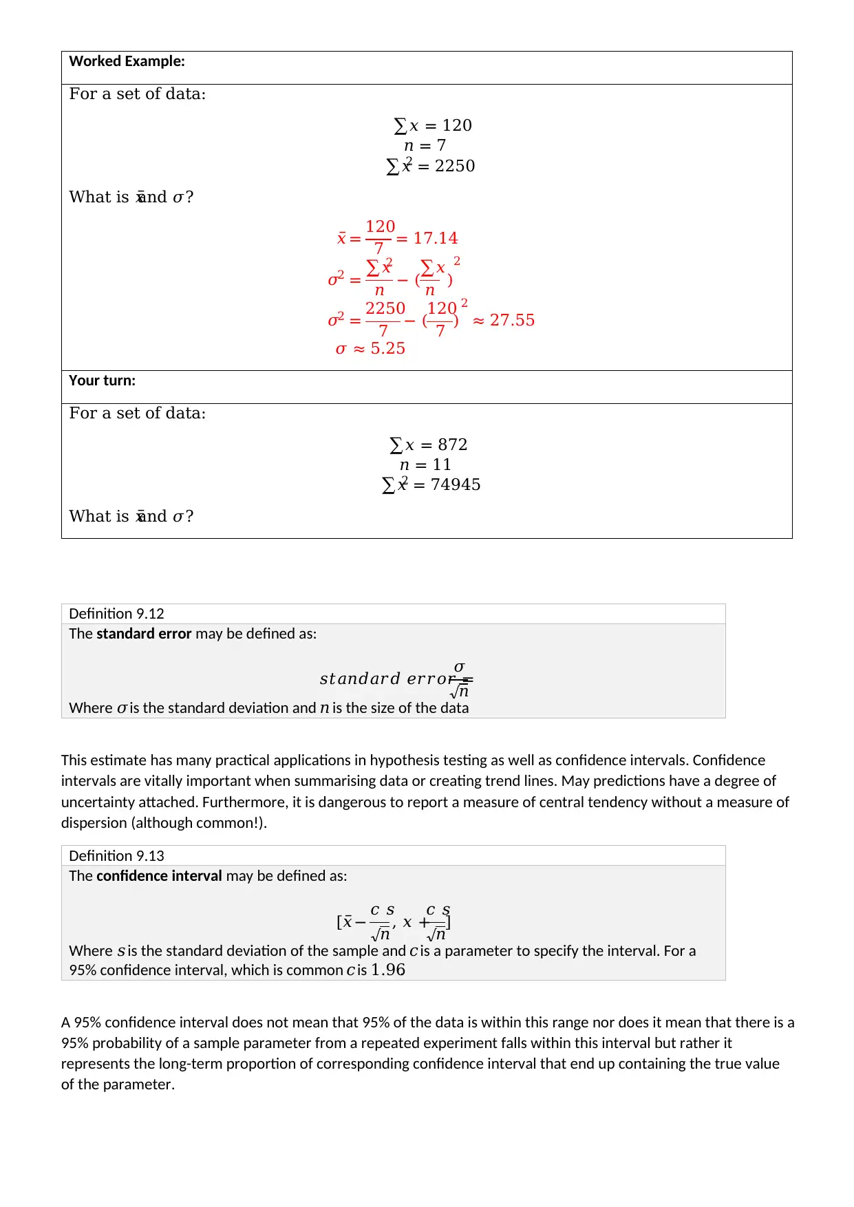
Worked Example:
For a set of data:
∑𝑥 = 120
𝑛 = 7
∑𝑥2 = 2250
What is 𝑥̅and 𝜎?
𝑥̅ = 120
7 = 17.14
𝜎2 = ∑𝑥2
𝑛 − (∑𝑥
𝑛 )
2
𝜎2 = 2250
7 − (120
7 )
2
≈ 27.55
𝜎 ≈ 5.25
Your turn:
For a set of data:
∑𝑥 = 872
𝑛 = 11
∑𝑥2 = 74945
What is 𝑥̅and 𝜎?
Definition 9.12
The standard error may be defined as:
𝑠𝑡𝑎𝑛𝑑𝑎𝑟𝑑 𝑒𝑟𝑟𝑜𝑟 =
𝜎
√𝑛
Where 𝜎is the standard deviation and 𝑛 is the size of the data
This estimate has many practical applications in hypothesis testing as well as confidence intervals. Confidence
intervals are vitally important when summarising data or creating trend lines. May predictions have a degree of
uncertainty attached. Furthermore, it is dangerous to report a measure of central tendency without a measure of
dispersion (although common!).
Definition 9.13
The confidence interval may be defined as:
[𝑥̅− 𝑐 𝑠
√𝑛, 𝑥 +
𝑐 𝑠
√𝑛]
Where 𝑠 is the standard deviation of the sample and 𝑐 is a parameter to specify the interval. For a
95% confidence interval, which is common 𝑐 is 1.96.
A 95% confidence interval does not mean that 95% of the data is within this range nor does it mean that there is a
95% probability of a sample parameter from a repeated experiment falls within this interval but rather it
represents the long-term proportion of corresponding confidence interval that end up containing the true value
of the parameter.
For a set of data:
∑𝑥 = 120
𝑛 = 7
∑𝑥2 = 2250
What is 𝑥̅and 𝜎?
𝑥̅ = 120
7 = 17.14
𝜎2 = ∑𝑥2
𝑛 − (∑𝑥
𝑛 )
2
𝜎2 = 2250
7 − (120
7 )
2
≈ 27.55
𝜎 ≈ 5.25
Your turn:
For a set of data:
∑𝑥 = 872
𝑛 = 11
∑𝑥2 = 74945
What is 𝑥̅and 𝜎?
Definition 9.12
The standard error may be defined as:
𝑠𝑡𝑎𝑛𝑑𝑎𝑟𝑑 𝑒𝑟𝑟𝑜𝑟 =
𝜎
√𝑛
Where 𝜎is the standard deviation and 𝑛 is the size of the data
This estimate has many practical applications in hypothesis testing as well as confidence intervals. Confidence
intervals are vitally important when summarising data or creating trend lines. May predictions have a degree of
uncertainty attached. Furthermore, it is dangerous to report a measure of central tendency without a measure of
dispersion (although common!).
Definition 9.13
The confidence interval may be defined as:
[𝑥̅− 𝑐 𝑠
√𝑛, 𝑥 +
𝑐 𝑠
√𝑛]
Where 𝑠 is the standard deviation of the sample and 𝑐 is a parameter to specify the interval. For a
95% confidence interval, which is common 𝑐 is 1.96.
A 95% confidence interval does not mean that 95% of the data is within this range nor does it mean that there is a
95% probability of a sample parameter from a repeated experiment falls within this interval but rather it
represents the long-term proportion of corresponding confidence interval that end up containing the true value
of the parameter.
⊘ This is a preview!⊘
Do you want full access?
Subscribe today to unlock all pages.
Trusted by 1+ million students worldwide
1 out of 34
Your All-in-One AI-Powered Toolkit for Academic Success.
+13062052269
info@desklib.com
Available 24*7 on WhatsApp / Email
![[object Object]](/_next/static/media/star-bottom.7253800d.svg)
Unlock your academic potential
Copyright © 2020–2026 A2Z Services. All Rights Reserved. Developed and managed by ZUCOL.