Computer Scheduling and Architecture Report: Algorithms Analysis

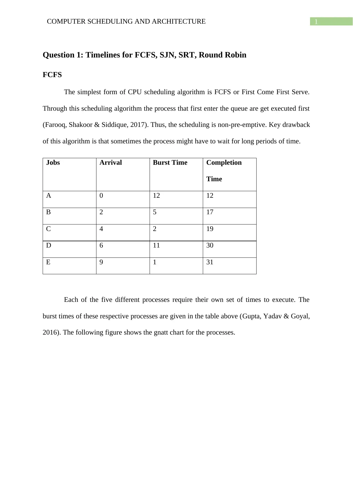
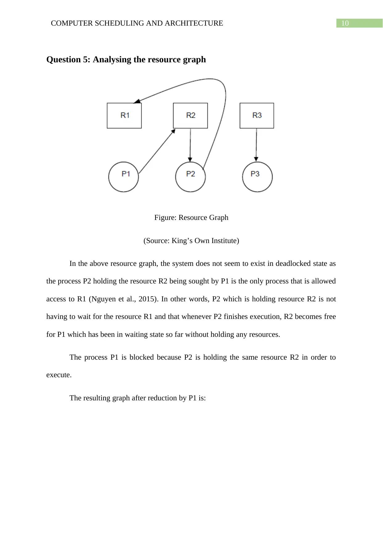
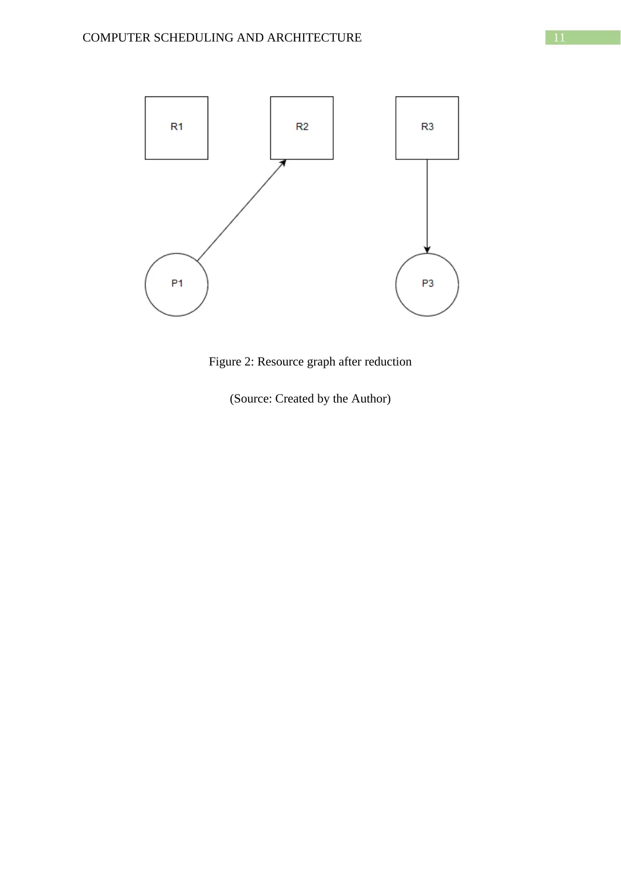
This report provides a comprehensive analysis of computer scheduling algorithms and their impact on system performance. It begins by examining the FCFS, SJN, SRT, and Round Robin scheduling algorithms, including their timelines and ready queue formation. The report calculates waiting time and turnaround time for each process under FCFS, SJN, SRT and Round Robin scheduling. Furthermore, it delves into the critical issue of deadlocks, discussing their causes, detection methods, and prevention strategies. The report explores various aspects of deadlock prevention, including mutual exclusion, no preemption, and circular wait conditions. A detailed analysis of a banking system scenario that uses lock, update, and unlock operations is provided, along with methods to avoid deadlocks. Finally, the report analyzes a resource graph to identify potential deadlocks and evaluate system states. The analysis includes a step-by-step evaluation to determine if the system exists in a deadlocked state, along with a visual representation of the resource graph after reduction by P1.

Running head: COMPUTER SCHEDULING AND ARCHITECTURE
Computer Scheduling and Architecture
Name of the Student
Name of the University
Author Note

1COMPUTER SCHEDULING AND ARCHITECTURE
Question 1: Timelines for FCFS, SJN, SRT, Round Robin
FCFS
The simplest form of CPU scheduling algorithm is FCFS or First Come First Serve.
Through this scheduling algorithm the process that first enter the queue are get executed first
(Farooq, Shakoor & Siddique, 2017). Thus, the scheduling is non-pre-emptive. Key drawback
of this algorithm is that sometimes the process might have to wait for long periods of time.
Jobs Arrival Burst Time Completion
Time
A 0 12 12
B 2 5 17
C 4 2 19
D 6 11 30
E 9 1 31
Each of the five different processes require their own set of times to execute. The
burst times of these respective processes are given in the table above (Gupta, Yadav & Goyal,
2016). The following figure shows the gnatt chart for the processes.

2COMPUTER SCHEDULING AND ARCHITECTURE
A B C D E
0 12 17 19 30 31
SJN
SJN or Shortest Job Next, also known as Shortest Job First (SJF) refers to the
scheduling algorithm by which the process with the shortest time of execution is selected
(Chugh, 2018). This is a greedy algorithm that has the advantage of having maximum
average waiting times among the rest of the algorithms. The downside of this algorithm being
occurrence of starvation due to repeated entry of shorter processes. Such problems can be
solved through the concept of aging. This algorithm is usually not feasible as the operating
system cannot know the burst times. A few methods to help determine the execution time, for
example the weighted average of prior times of execution of the particular set of process. As
a result, SJN is only considered suited for specialized scenarios that can offer very accurate
estimates of execution times.
The algorithm can be explained in two simple steps:
1. Sort all the processes in increasing order of burst times
2. Apply the FCFS scheduling algorithm
Jobs Arrival Burst Time
A 0 12
E 9 1
C 4 2
B 2 5
D 6 11

3COMPUTER SCHEDULING AND ARCHITECTURE
The arrival times are very important. Since only 1 process is available at the start - process A,
automatically becomes the shortest process.
At time 2, process B arrives but process A is also running. Since they are not pre-empted,
therefore even if process B is shorter it needs to wait till process A completes execution.
At time 4, process C arrives which is now the shortest among the processes but process A is
yet to complete execution.
At time 6, process D arrives but process C continues to be the shortest process and process A
is still in execution.
At time 9, process E arrives and becomes the shortest process. Therefore, after time 12 when
process A finishes, process E will be executed first.
SRT
SRT or Shortest Remaining Time is the scheduling algorithm that is considered as the
pre-emptive version of shortest job next (SJN) (Almakdi, Aleisa & Alshehri, 2015). In SRT
processes having the smallest execution times are run first, similar to SJN. However, in SJN
once a process begins running, it completes execution but in SRT these running processes get
pre-empted by other processes having shorter execution times.
Jobs Arrival Burst Time
A 0 12
B 2 5
C 4 2
D 6 11
E 9 1

4COMPUTER SCHEDULING AND ARCHITECTURE
For the processes mentioned in the table above the ready can look like the following:
A B C B E A D
0 2 4 5 8 9 19 30
Here A being the starting process is executed first.
B is a shorter process so when B enters the queue at time 2 it pre-empts process A which
required (12-2 = 10) milliseconds more CPU time.
C enters the queue at time 4 and being shorter than B, pre-empts process B, which requires
(5-2 = 3) milliseconds.
After process C completes execution at time 6, D arrives but B is shorter having 3
millisecond of CPU time left.
Then, after B finishes execution at time 9, process E enters queue and being the shortest
process takes over CPU time ahead of processes A and D.
After E finishes execution, process A requiring 10 milliseconds CPU time – less than 11 of D
enters execution.
Only after process A finishes D gets to run.
Round Robin (Time quantum 3)
The other scheduling algorithm that is Round Robin Scheduling algorithm concerns
with allocating smaller amounts of CPU time to every process at a given time up to which the
process runs (Siahaan, 2016). These small units of CPU time are called CPU time slice or

5COMPUTER SCHEDULING AND ARCHITECTURE
time quantum. Here, when the time slice expires the process gets pre-empted by the next
process in a circular queue.
Jobs Arrival Burst Time
A 0 12
B 2 5
C 4 2
D 6 11
E 9 1
For the processes given in the table above, the gnatt chart for round robin scheduling with
time quantum = 3 can be:
A B C B E D A D A D A D
0 3 6 8 11 12 15 18 21 24 27 30 32
Here the time quantum of 3 is assigned to all the five processes in the table which the
processes cannot exceed but can vacate CPU early if execution is finished. The chart above
clearly elaborates the scheduling mechanism for the given processes.
Question 2: Waiting time and Turn Around time
Scheduling of processes are conducted so that the processes are executed on time by
the operating system or in CPU scheduling. The two key times are arrival time and
completion time. Arrival Time is the time when a particular process enters the queue (Dash &
Samantra, 2016). Completion Time is the time at which the process executes completely
(Fataniya & Patel, 2018). From these the waiting time and the turn around time of processes
are calculated. Turn around time is taken as the difference between the completion and arrival

6COMPUTER SCHEDULING AND ARCHITECTURE
times of processes (Ahmad, Ahmad & Mirdha, 2017). Waiting time of process is considered
to be the difference between the turn around time and the Burst time (Razaque et all., 2016).
For the above set of processes, these times can be calculated as:
Turn Around Time of Process A = 12 – 0 = 12
Turn Around Time of Process B = 17 – 2 = 15
Turn Around Time of Process C = 19 – 4 = 15
Turn Around Time of Process D = 30 – 6 = 24
Turn Around Time of Process E = 31 – 9 = 22
Waiting Time of Process, A = 12 – 12 = 0
Waiting Time of Process B = 15 – 5 = 10
Waiting Time of Process C = 15 – 2 = 13
Waiting Time of Process D = 24 – 11 = 13
Waiting Time of Process E = 22 – 1 = 21
Question 3: Avoiding recurring deadlocks and steps to mitigate deadlocks
To identify the reasons for existence of deadlocks, the operating system should be
analysed and checked for the following events:
Detection – Processes that examine state of the operating system so as to decide if any
deadlock exists or not.
Directed graphs – Graphic models that are used to represent the way resources are being
allocated.

7COMPUTER SCHEDULING AND ARCHITECTURE
Livelock – An already locked system multiple processes continuously blocking forward
progress of other processes without even progressing forward themselves (Conserva Filho et
al., 2018). This is almost akin to a deadlock except for the processes are not blocked or exist
in waiting state. That is the processes are undergoing continuous changes without making
progress.
Locking – These are techniques used for guaranteeing data integrity in databases by which
users can lock other users while working with the databases.
Mutual Exclusion – Among the four conditions for deadlock to occur, mutual exclusion is
one. Here only one process is allowed to have access to resources.
No pre-emption – Also among the four conditions for deadlocks to occur (Abdoos, 2017).
Here the process is allowed for holding the resource till the time it waits for other processes
to finish executions.
Prevention – The strategy for operating systems in which resources need to be managed such
that the respective conditions for developing deadlocks are not held.
Process synchronization – The requirement of algorithms for resolving conflicts among
processors in multiprocessing environments or needs of ensuring that the respective events
take place in proper order even if they get carried out by multiple processes.
Race – This condition happens when a synchronization problem is noted between processes
trying to access the same resources.
Recovery – This refers to the steps that need to be taken when deadlock get detected by
ending the circle involving waiting processes.

8COMPUTER SCHEDULING AND ARCHITECTURE
Resource holding – Among the four conditions for deadlock to occur, here processes refuse
to give up resources they are holding till their execution gets completed, despite not using the
resources as they are waiting for other resources.
Safe state – The sate at which the operating system has enough resources available for
guaranteeing execution of one process being run.
Spooling – It refers to the technique developed for speeding up I/O by collecting them in files
on the disk (Silberschatz, Gagne & Galvin, 2018). These can involve either inputs from
slower devices or output to slower output devices.
Starvation – This can result from conservative resource allocation processes such that a single
process is getting blocked from completing execution as it waits for resources that may never
become available.
Unsafe state – Refers to the situation where the system contains very few resources for
guaranteeing completion of even one process present of the system.
Victim – Refers to an expendable task for removing systems from deadlocked state so as to
share more resources to waiting processes thus resolving the deadlock.
Circular Wait – The last remaining of the four conditions for deadlocks to occur. Concerns
with formation of circular chains of multiple processes each of which waiting for resources
held by the other members in the chain (Liu & Chen, 2016). Thus, this can lead into
deadlocks.

9COMPUTER SCHEDULING AND ARCHITECTURE
Question 4: Evaluating deadlock prevention in a banking system that uses
steps – lock, update and unlock
lock A(i); lock A(j);
update A(i); update A(j);
unlock A(i); unlock A(j);
The processes lock A(i), lock A(j); update A(i), update A(j) and unlock A(i), unlock
A(j) are similar set of commands running parallelly to operate with account numbers by
accessing currently available resources through matrices A(i) and A(j) (Yao, Yin & Wu,
2016). Since the same resources are being utilized at the same time by two different
processes, there is high chance of encountering deadlocks if sufficient resources are not
available.
The numbering request policy if implemented can prevent deadlocks where the
number of accounts is dynamic (Gupta & Gore, 2016). This is because by reducing the
number of lock attempts when such load is not needed valuable resources can be freed up and
this can then be allocated to processes seeking resources and existing in waiting state. This
way deadlocks can be prevented.

10COMPUTER SCHEDULING AND ARCHITECTURE
Question 5: Analysing the resource graph
Figure: Resource Graph
(Source: King’s Own Institute)
In the above resource graph, the system does not seem to exist in deadlocked state as
the process P2 holding the resource R2 being sought by P1 is the only process that is allowed
access to R1 (Nguyen et al., 2015). In other words, P2 which is holding resource R2 is not
having to wait for the resource R1 and that whenever P2 finishes execution, R2 becomes free
for P1 which has been in waiting state so far without holding any resources.
The process P1 is blocked because P2 is holding the same resource R2 in order to
execute.
The resulting graph after reduction by P1 is:

11COMPUTER SCHEDULING AND ARCHITECTURE
Figure 2: Resource graph after reduction
(Source: Created by the Author)