Computing Assignment 1: Statistical Analysis and Hypothesis Testing
VerifiedAdded on 2021/06/14
|12
|1566
|57
Homework Assignment
AI Summary
This document presents a comprehensive solution to Computing Assignment 1, focusing on statistical analysis and hypothesis testing. The assignment involves analyzing a sample statistical report, identifying variable types (categorical and quantitative), and calculating summary statistics, including measures of central tendency and variation. The solution includes the creation and interpretation of contingency tables, stacked bar graphs, and back-to-back histograms to visualize data relationships. Hypothesis testing is performed to assess the difference in proportions between groups and the difference between means, with p-values calculated and interpreted. Z-scores are computed and used for rank comparisons. The assignment also covers the relationship between variables, scatter plots, and the interpretation of findings in a business context. The solution provides a detailed explanation of the statistical methods and their application to the given data, including an analysis of the expected and actual ranks.
Computing Assignment 1
COMPUTING ASSIGNMENT
Name
Course Number
Date
Faculty Number
Allocated Sample: 443
COMPUTING ASSIGNMENT
Name
Course Number
Date
Faculty Number
Allocated Sample: 443
Paraphrase This Document
Need a fresh take? Get an instant paraphrase of this document with our AI Paraphraser
Computing Assignment 2
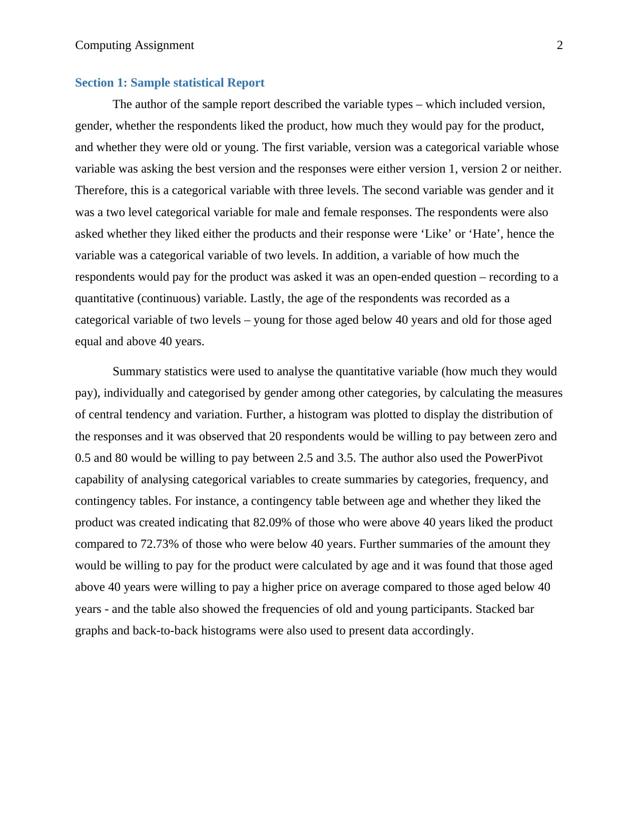
Section 1: Sample statistical Report
The author of the sample report described the variable types – which included version,
gender, whether the respondents liked the product, how much they would pay for the product,
and whether they were old or young. The first variable, version was a categorical variable whose
variable was asking the best version and the responses were either version 1, version 2 or neither.
Therefore, this is a categorical variable with three levels. The second variable was gender and it
was a two level categorical variable for male and female responses. The respondents were also
asked whether they liked either the products and their response were ‘Like’ or ‘Hate’, hence the
variable was a categorical variable of two levels. In addition, a variable of how much the
respondents would pay for the product was asked it was an open-ended question – recording to a
quantitative (continuous) variable. Lastly, the age of the respondents was recorded as a
categorical variable of two levels – young for those aged below 40 years and old for those aged
equal and above 40 years.
Summary statistics were used to analyse the quantitative variable (how much they would
pay), individually and categorised by gender among other categories, by calculating the measures
of central tendency and variation. Further, a histogram was plotted to display the distribution of
the responses and it was observed that 20 respondents would be willing to pay between zero and
0.5 and 80 would be willing to pay between 2.5 and 3.5. The author also used the PowerPivot
capability of analysing categorical variables to create summaries by categories, frequency, and
contingency tables. For instance, a contingency table between age and whether they liked the
product was created indicating that 82.09% of those who were above 40 years liked the product
compared to 72.73% of those who were below 40 years. Further summaries of the amount they
would be willing to pay for the product were calculated by age and it was found that those aged
above 40 years were willing to pay a higher price on average compared to those aged below 40
years - and the table also showed the frequencies of old and young participants. Stacked bar
graphs and back-to-back histograms were also used to present data accordingly.
Computing Assignment 3
Section 2
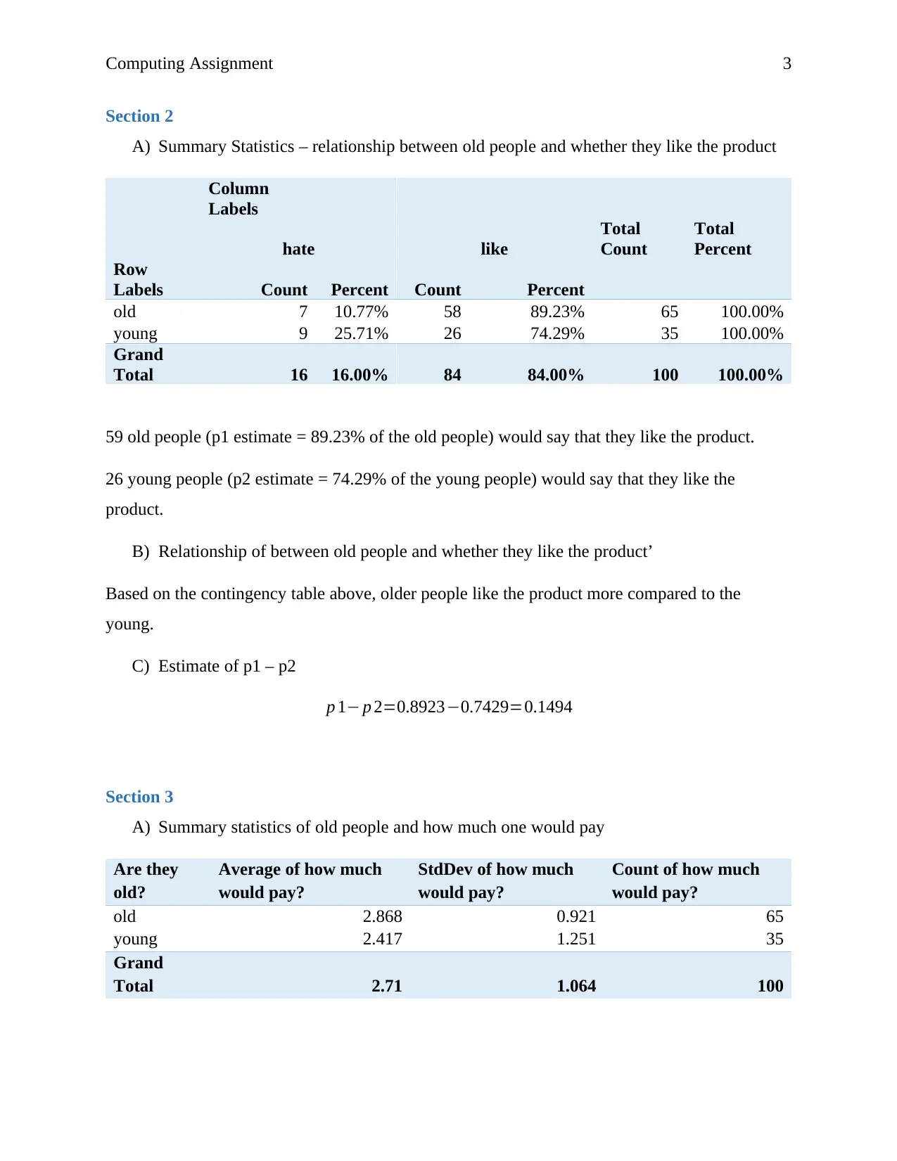
A) Summary Statistics – relationship between old people and whether they like the product
Column
Labels
hate like
Total
Count
Total
Percent
Row
Labels Count Percent Count Percent
old 7 10.77% 58 89.23% 65 100.00%
young 9 25.71% 26 74.29% 35 100.00%
Grand
Total 16 16.00% 84 84.00% 100 100.00%
59 old people (p1 estimate = 89.23% of the old people) would say that they like the product.
26 young people (p2 estimate = 74.29% of the young people) would say that they like the
product.
B) Relationship of between old people and whether they like the product’
Based on the contingency table above, older people like the product more compared to the
young.
C) Estimate of p1 – p2
p 1− p 2=0.8923−0.7429=0.1494
Section 3
A) Summary statistics of old people and how much one would pay
Are they
old?
Average of how much
would pay?
StdDev of how much
would pay?
Count of how much
would pay?
old 2.868 0.921 65
young 2.417 1.251 35
Grand
Total 2.71 1.064 100
⊘ This is a preview!⊘
Do you want full access?
Subscribe today to unlock all pages.

Trusted by 1+ million students worldwide
Computing Assignment 4
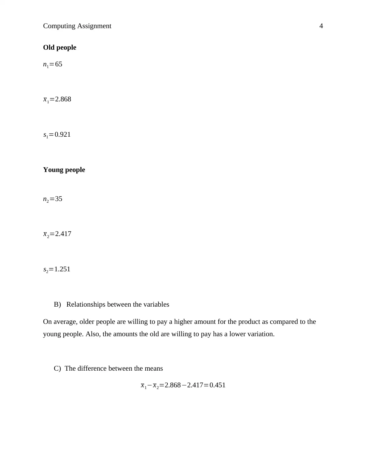
Old people
n1=65
x1=2.868
s1=0.921
Young people
n2 =35
x2=2.417
s2=1.251
B) Relationships between the variables
On average, older people are willing to pay a higher amount for the product as compared to the
young people. Also, the amounts the old are willing to pay has a lower variation.
C) The difference between the means
x1−x2=2.868−2.417=0.451
Paraphrase This Document
Need a fresh take? Get an instant paraphrase of this document with our AI Paraphraser
Computing Assignment 5
Section 4
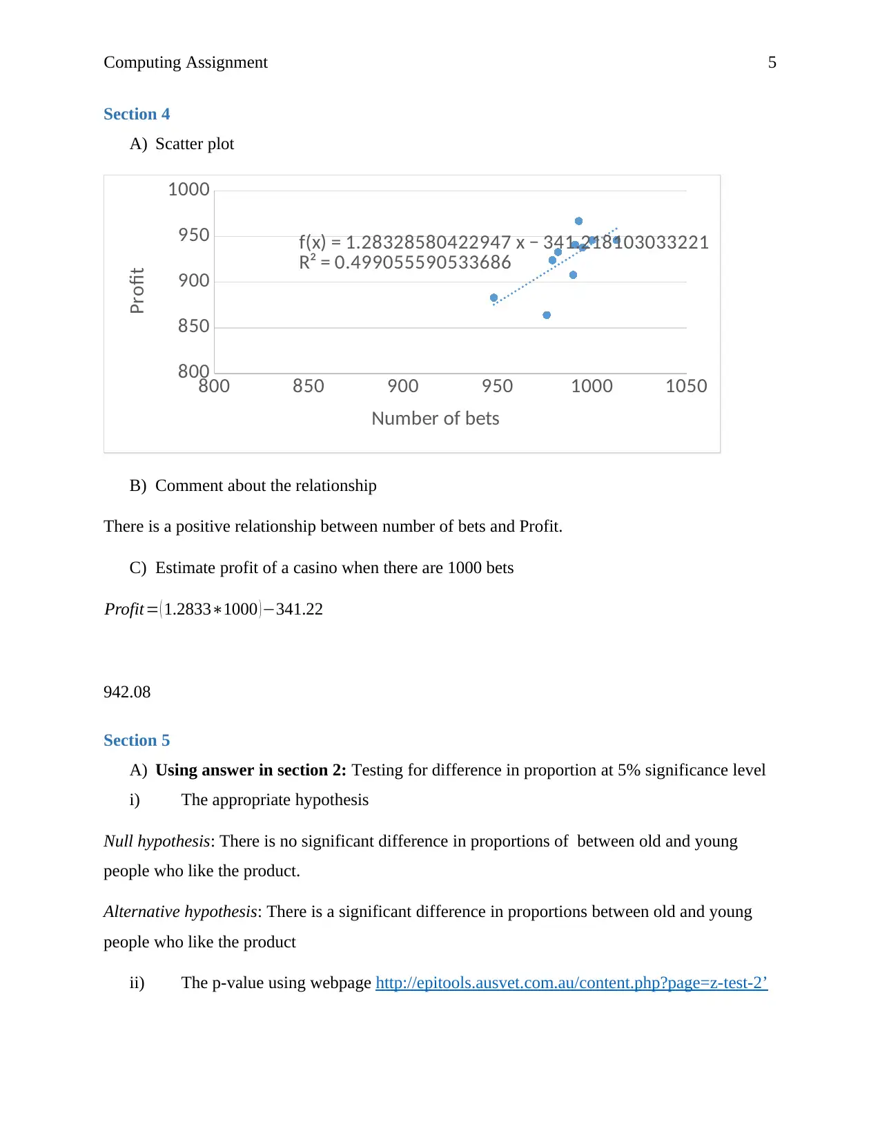
A) Scatter plot
800 850 900 950 1000 1050
800
850
900
950
1000
f(x) = 1.28328580422947 x − 341.218103033221
R² = 0.499055590533686
Number of bets
Profit
B) Comment about the relationship
There is a positive relationship between number of bets and Profit.
C) Estimate profit of a casino when there are 1000 bets
Profit= ( 1.2833∗1000 )−341.22
942.08
Section 5
A) Using answer in section 2: Testing for difference in proportion at 5% significance level
i) The appropriate hypothesis
Null hypothesis: There is no significant difference in proportions of between old and young
people who like the product.
Alternative hypothesis: There is a significant difference in proportions between old and young
people who like the product
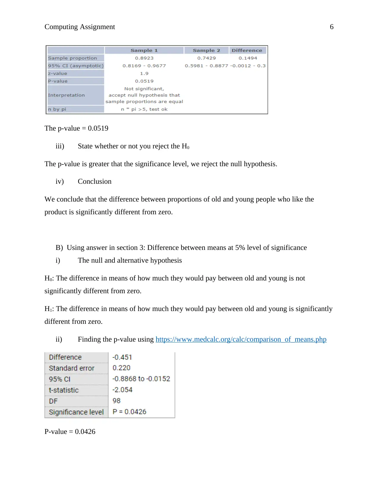
ii) The p-value using webpage http://epitools.ausvet.com.au/content.php?page=z-test-2’
Computing Assignment 6
The p-value = 0.0519
iii) State whether or not you reject the H0
The p-value is greater that the significance level, we reject the null hypothesis.
iv) Conclusion
We conclude that the difference between proportions of old and young people who like the
product is significantly different from zero.
B) Using answer in section 3: Difference between means at 5% level of significance
i) The null and alternative hypothesis
H0: The difference in means of how much they would pay between old and young is not
significantly different from zero.
H1: The difference in means of how much they would pay between old and young is significantly
different from zero.
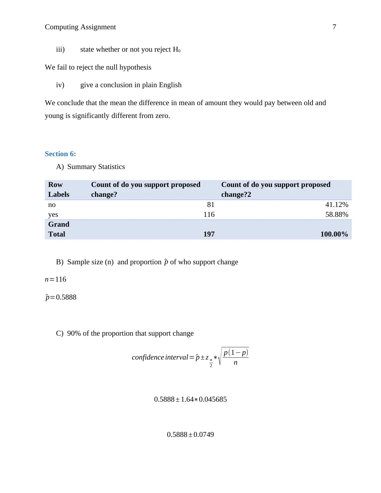
ii) Finding the p-value using https://www.medcalc.org/calc/comparison_of_means.php
P-value = 0.0426
⊘ This is a preview!⊘
Do you want full access?
Subscribe today to unlock all pages.

Trusted by 1+ million students worldwide
Computing Assignment 7
iii) state whether or not you reject H0
We fail to reject the null hypothesis
iv) give a conclusion in plain English
We conclude that the mean the difference in mean of amount they would pay between old and
young is significantly different from zero.
Section 6:
A) Summary Statistics
Row
Labels
Count of do you support proposed
change?
Count of do you support proposed
change?2
no 81 41.12%
yes 116 58.88%
Grand
Total 197 100.00%
B) Sample size (n) and proportion ^p of who support change
n=116
^p=0.5888
C) 90% of the proportion that support change
confidence interval= ^p ± z ∝
2
∗
√ p(1− p)
n
0.5888 ± 1.64∗0.045685
0.5888 ± 0.0749
Paraphrase This Document
Need a fresh take? Get an instant paraphrase of this document with our AI Paraphraser
Computing Assignment 8
lower bound=0.5139
upper bound=0.6637
Section 7:
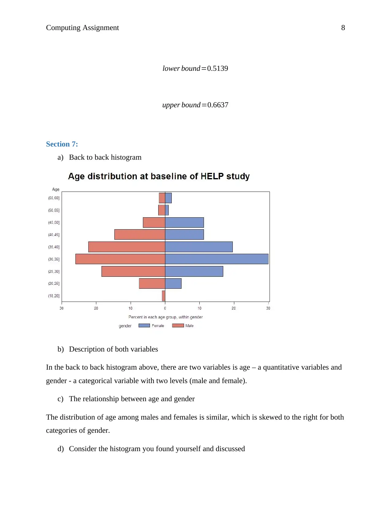
a) Back to back histogram
b) Description of both variables
In the back to back histogram above, there are two variables is age – a quantitative variables and
gender - a categorical variable with two levels (male and female).
c) The relationship between age and gender
The distribution of age among males and females is similar, which is skewed to the right for both
categories of gender.
d) Consider the histogram you found yourself and discussed
Computing Assignment 9
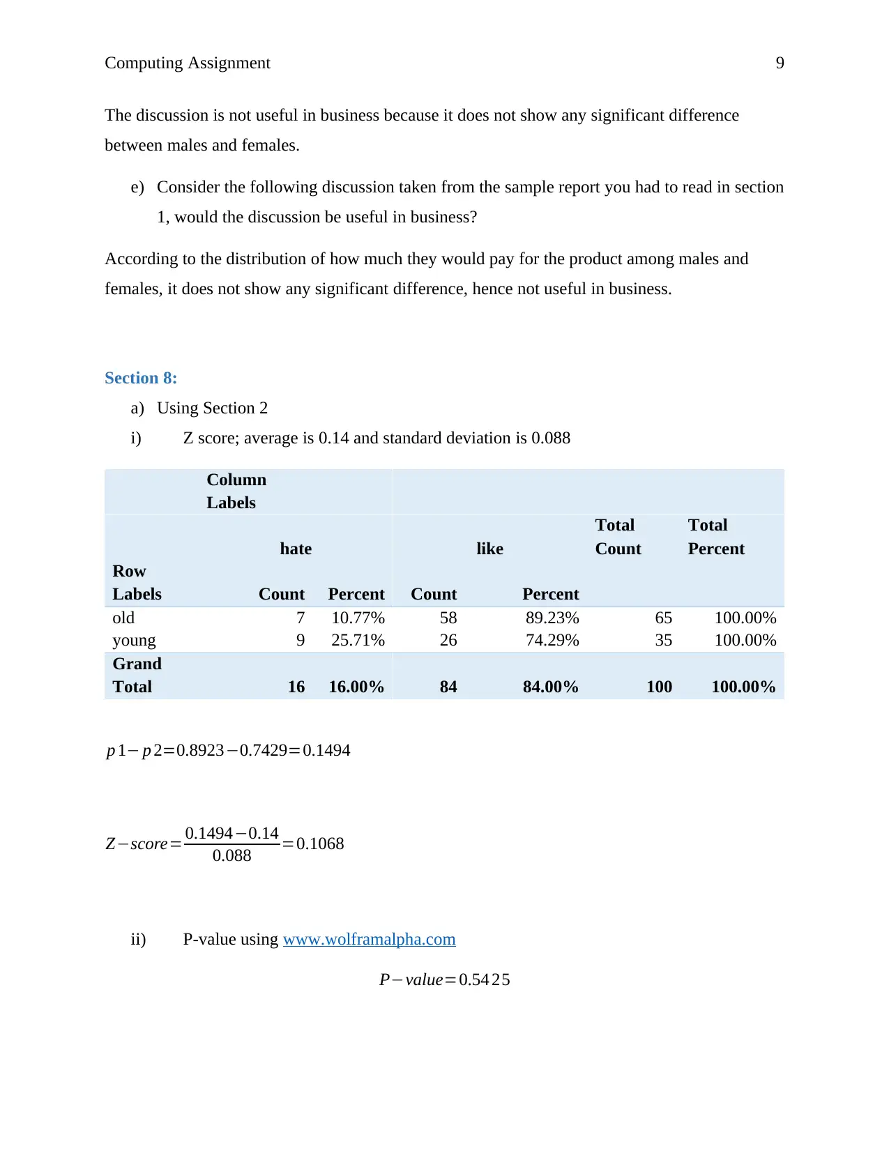
The discussion is not useful in business because it does not show any significant difference
between males and females.
e) Consider the following discussion taken from the sample report you had to read in section
1, would the discussion be useful in business?
According to the distribution of how much they would pay for the product among males and
females, it does not show any significant difference, hence not useful in business.
Section 8:
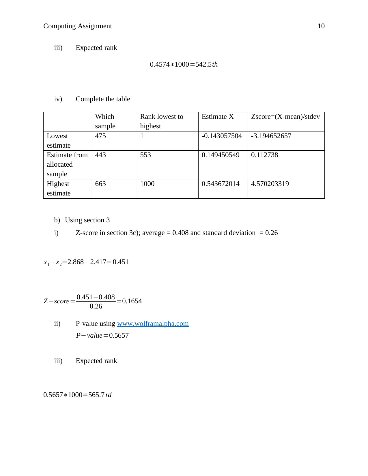
a) Using Section 2
i) Z score; average is 0.14 and standard deviation is 0.088
Column
Labels
hate like
Total
Count
Total
Percent
Row
Labels Count Percent Count Percent
old 7 10.77% 58 89.23% 65 100.00%
young 9 25.71% 26 74.29% 35 100.00%
Grand
Total 16 16.00% 84 84.00% 100 100.00%
p 1− p 2=0.8923−0.7429=0.1494
Z−score= 0.1494−0.14
0.088 =0.1068
ii) P-value using www.wolframalpha.com
P−value=0.54 25
⊘ This is a preview!⊘
Do you want full access?
Subscribe today to unlock all pages.

Trusted by 1+ million students worldwide
Computing Assignment 10
iii) Expected rank
0.4574∗1000=542.5th
iv) Complete the table
Which
sample
Rank lowest to
highest
Estimate X Zscore=(X-mean)/stdev
Lowest
estimate
475 1 -0.143057504 -3.194652657
Estimate from
allocated
sample
443 553 0.149450549 0.112738
Highest
estimate
663 1000 0.543672014 4.570203319
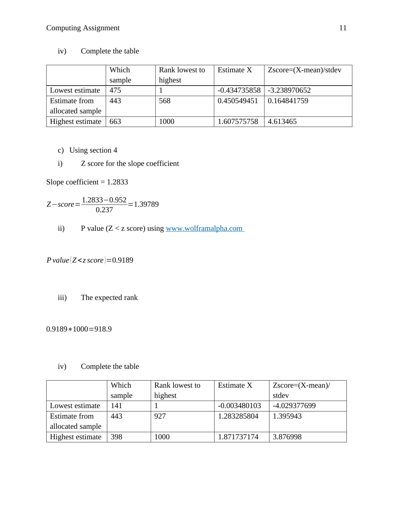
b) Using section 3
i) Z-score in section 3c); average = 0.408 and standard deviation = 0.26
x1−x2=2.868−2.417=0.451
Z−score= 0.451−0.408
0.26 =0.1654
ii) P-value using www.wolframalpha.com
P−value=0.5657
iii) Expected rank
0.5657∗1000=565.7 rd
iii) Expected rank
0.4574∗1000=542.5th
iv) Complete the table
Which
sample
Rank lowest to
highest
Estimate X Zscore=(X-mean)/stdev
Lowest
estimate
475 1 -0.143057504 -3.194652657
Estimate from
allocated
sample
443 553 0.149450549 0.112738
Highest
estimate
663 1000 0.543672014 4.570203319
b) Using section 3
i) Z-score in section 3c); average = 0.408 and standard deviation = 0.26
x1−x2=2.868−2.417=0.451
Z−score= 0.451−0.408
0.26 =0.1654
ii) P-value using www.wolframalpha.com
P−value=0.5657
iii) Expected rank
0.5657∗1000=565.7 rd
Paraphrase This Document
Need a fresh take? Get an instant paraphrase of this document with our AI Paraphraser
Computing Assignment 11
iv) Complete the table
Which
sample
Rank lowest to
highest
Estimate X Zscore=(X-mean)/stdev
Lowest estimate 475 1 -0.434735858 -3.238970652
Estimate from
allocated sample
443 568 0.450549451 0.164841759
Highest estimate 663 1000 1.607575758 4.613465
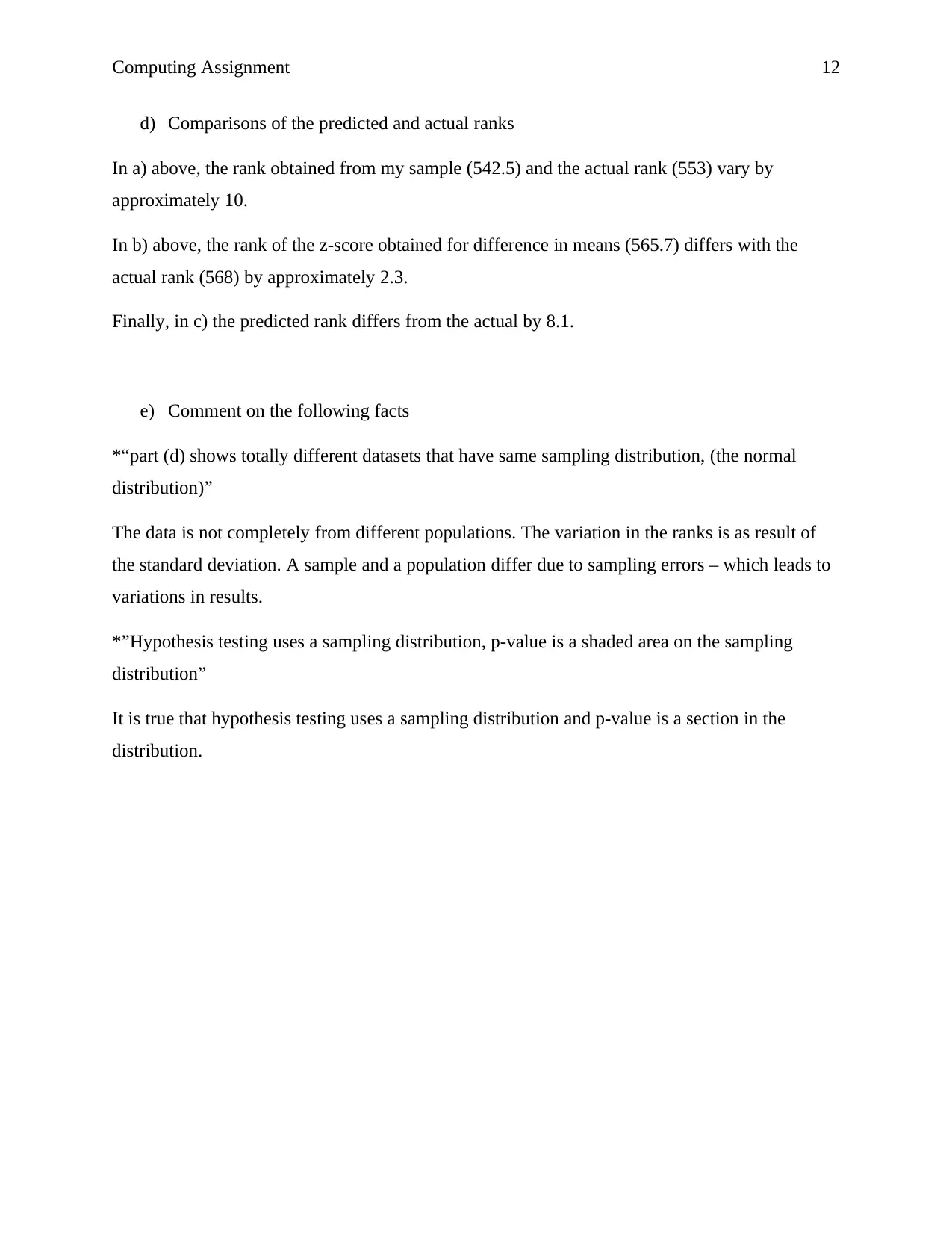
c) Using section 4
i) Z score for the slope coefficient
Slope coefficient = 1.2833
Z−score= 1.2833−0.952
0.237 =1.39789
ii) P value (Z < z score) using www.wolframalpha.com
P value ( Z <z score )=0.9189
iii) The expected rank
0.9189∗1000=918.9
iv) Complete the table
Which
sample
Rank lowest to
highest
Estimate X Zscore=(X-mean)/
stdev
Lowest estimate 141 1 -0.003480103 -4.029377699
Estimate from
allocated sample
443 927 1.283285804 1.395943
Highest estimate 398 1000 1.871737174 3.876998
iv) Complete the table
Which
sample
Rank lowest to
highest
Estimate X Zscore=(X-mean)/stdev
Lowest estimate 475 1 -0.434735858 -3.238970652
Estimate from
allocated sample
443 568 0.450549451 0.164841759
Highest estimate 663 1000 1.607575758 4.613465
c) Using section 4
i) Z score for the slope coefficient
Slope coefficient = 1.2833
Z−score= 1.2833−0.952
0.237 =1.39789
ii) P value (Z < z score) using www.wolframalpha.com
P value ( Z <z score )=0.9189
iii) The expected rank
0.9189∗1000=918.9
iv) Complete the table
Which
sample
Rank lowest to
highest
Estimate X Zscore=(X-mean)/
stdev
Lowest estimate 141 1 -0.003480103 -4.029377699
Estimate from
allocated sample
443 927 1.283285804 1.395943
Highest estimate 398 1000 1.871737174 3.876998
Computing Assignment 12
d) Comparisons of the predicted and actual ranks
In a) above, the rank obtained from my sample (542.5) and the actual rank (553) vary by
approximately 10.
In b) above, the rank of the z-score obtained for difference in means (565.7) differs with the
actual rank (568) by approximately 2.3.
Finally, in c) the predicted rank differs from the actual by 8.1.
e) Comment on the following facts
*“part (d) shows totally different datasets that have same sampling distribution, (the normal
distribution)”
The data is not completely from different populations. The variation in the ranks is as result of
the standard deviation. A sample and a population differ due to sampling errors – which leads to
variations in results.
*”Hypothesis testing uses a sampling distribution, p-value is a shaded area on the sampling
distribution”
It is true that hypothesis testing uses a sampling distribution and p-value is a section in the
distribution.
⊘ This is a preview!⊘
Do you want full access?
Subscribe today to unlock all pages.

Trusted by 1+ million students worldwide
1 out of 12
Related Documents
Your All-in-One AI-Powered Toolkit for Academic Success.
+13062052269
info@desklib.com
Available 24*7 on WhatsApp / Email
![[object Object]](/_next/static/media/star-bottom.7253800d.svg)
Unlock your academic potential
Copyright © 2020–2026 A2Z Services. All Rights Reserved. Developed and managed by ZUCOL.


