Consolidation Computations Report
VerifiedAdded on 2020/03/23
|9
|992
|44
Report
AI Summary
This report presents detailed consolidation computations performed on a saturated clay sample from Brisbane. It includes effective stress analysis, void ratio calculations, and the impact of soil thickness on consolidation rates. The report also discusses the relationship between pore pressure and consolidation settlement, along with seepage quantity calculations for a homogenous soil layer. References are provided for further reading.
Consolidation Computations 1
CONSOLIDATION COMPUTATIONS
Name
Professor
University
City, State
Date
CONSOLIDATION COMPUTATIONS
Name
Professor
University
City, State
Date
Paraphrase This Document
Need a fresh take? Get an instant paraphrase of this document with our AI Paraphraser
Consolidation Computations 2
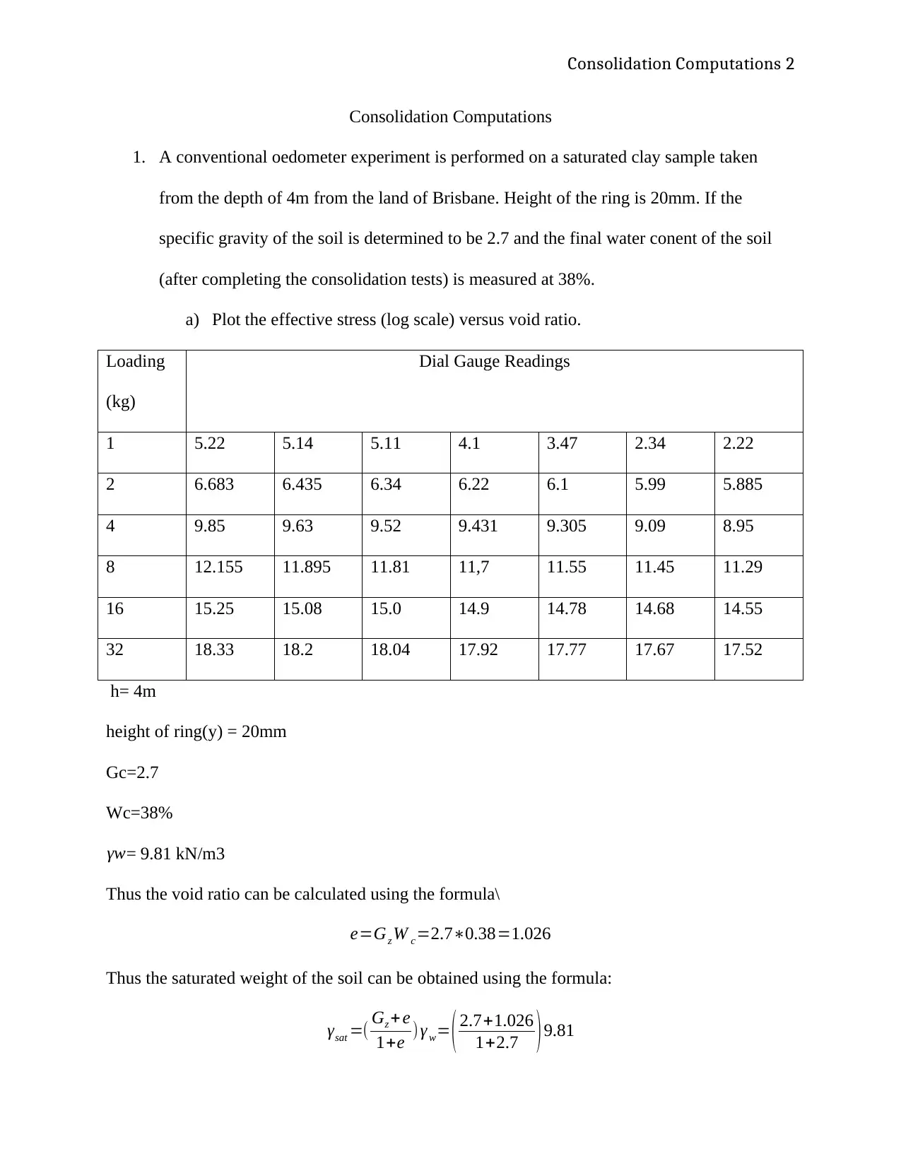
Consolidation Computations
1. A conventional oedometer experiment is performed on a saturated clay sample taken
from the depth of 4m from the land of Brisbane. Height of the ring is 20mm. If the
specific gravity of the soil is determined to be 2.7 and the final water conent of the soil
(after completing the consolidation tests) is measured at 38%.
a) Plot the effective stress (log scale) versus void ratio.
Loading
(kg)
Dial Gauge Readings
1 5.22 5.14 5.11 4.1 3.47 2.34 2.22
2 6.683 6.435 6.34 6.22 6.1 5.99 5.885
4 9.85 9.63 9.52 9.431 9.305 9.09 8.95
8 12.155 11.895 11.81 11,7 11.55 11.45 11.29
16 15.25 15.08 15.0 14.9 14.78 14.68 14.55
32 18.33 18.2 18.04 17.92 17.77 17.67 17.52
h= 4m
height of ring(y) = 20mm
Gc=2.7
Wc=38%
γw= 9.81 kN/m3
Thus the void ratio can be calculated using the formula\
e=Gz W c=2.7∗0.38=1.026
Thus the saturated weight of the soil can be obtained using the formula:
γsat =( Gz + e
1+e ) γ w= ( 2.7+1.026
1+2.7 )9.81
Consolidation Computations 3
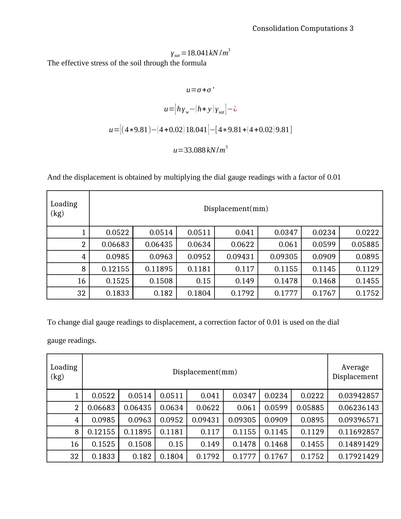
γsat =18.041kN /m3
The effective stress of the soil through the formula
u=σ +σ '
u= [ h γ w− ( h+ y ) γsat ] −¿
u= [( 4∗9.81)− ( 4 +0.02 ) 18.041 ]−[4∗9.81+ ( 4 +0.02 ) 9.81]
u=33.088 kN /m3
And the displacement is obtained by multiplying the dial gauge readings with a factor of 0.01
Loading
(kg) Displacement(mm)
1 0.0522 0.0514 0.0511 0.041 0.0347 0.0234 0.0222
2 0.06683 0.06435 0.0634 0.0622 0.061 0.0599 0.05885
4 0.0985 0.0963 0.0952 0.09431 0.09305 0.0909 0.0895
8 0.12155 0.11895 0.1181 0.117 0.1155 0.1145 0.1129
16 0.1525 0.1508 0.15 0.149 0.1478 0.1468 0.1455
32 0.1833 0.182 0.1804 0.1792 0.1777 0.1767 0.1752
To change dial gauge readings to displacement, a correction factor of 0.01 is used on the dial
gauge readings.
Loading
(kg) Displacement(mm) Average
Displacement
1 0.0522 0.0514 0.0511 0.041 0.0347 0.0234 0.0222 0.03942857
2 0.06683 0.06435 0.0634 0.0622 0.061 0.0599 0.05885 0.06236143
4 0.0985 0.0963 0.0952 0.09431 0.09305 0.0909 0.0895 0.09396571
8 0.12155 0.11895 0.1181 0.117 0.1155 0.1145 0.1129 0.11692857
16 0.1525 0.1508 0.15 0.149 0.1478 0.1468 0.1455 0.14891429
32 0.1833 0.182 0.1804 0.1792 0.1777 0.1767 0.1752 0.17921429
⊘ This is a preview!⊘
Do you want full access?
Subscribe today to unlock all pages.
Trusted by 1+ million students worldwide
Consolidation Computations 4
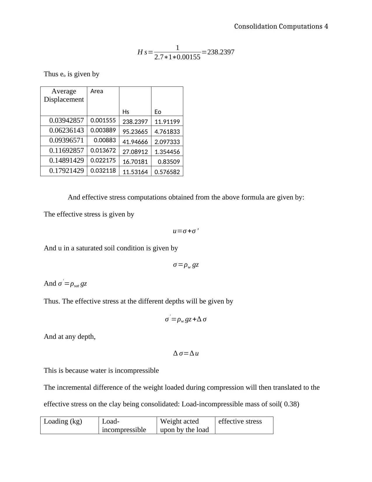
H s= 1
2.7∗1∗0.00155 =238.2397
Thus eo is given by
Average
Displacement
Area
Hs Eo
0.03942857 0.001555 238.2397 11.91199
0.06236143 0.003889 95.23665 4.761833
0.09396571 0.00883 41.94666 2.097333
0.11692857 0.013672 27.08912 1.354456
0.14891429 0.022175 16.70181 0.83509
0.17921429 0.032118 11.53164 0.576582
And effective stress computations obtained from the above formula are given by:
The effective stress is given by
u=σ +σ '
And u in a saturated soil condition is given by
σ =ρw gz
And σ '=ρsat gz
Thus. The effective stress at the different depths will be given by
σ '=ρw gz +∆ σ
And at any depth,
∆ σ=∆ u
This is because water is incompressible
The incremental difference of the weight loaded during compression will then translated to the
effective stress on the clay being consolidated: Load-incompressible mass of soil( 0.38)
Loading (kg) Load-
incompressible
Weight acted
upon by the load
effective stress
Paraphrase This Document
Need a fresh take? Get an instant paraphrase of this document with our AI Paraphraser
Consolidation Computations 5
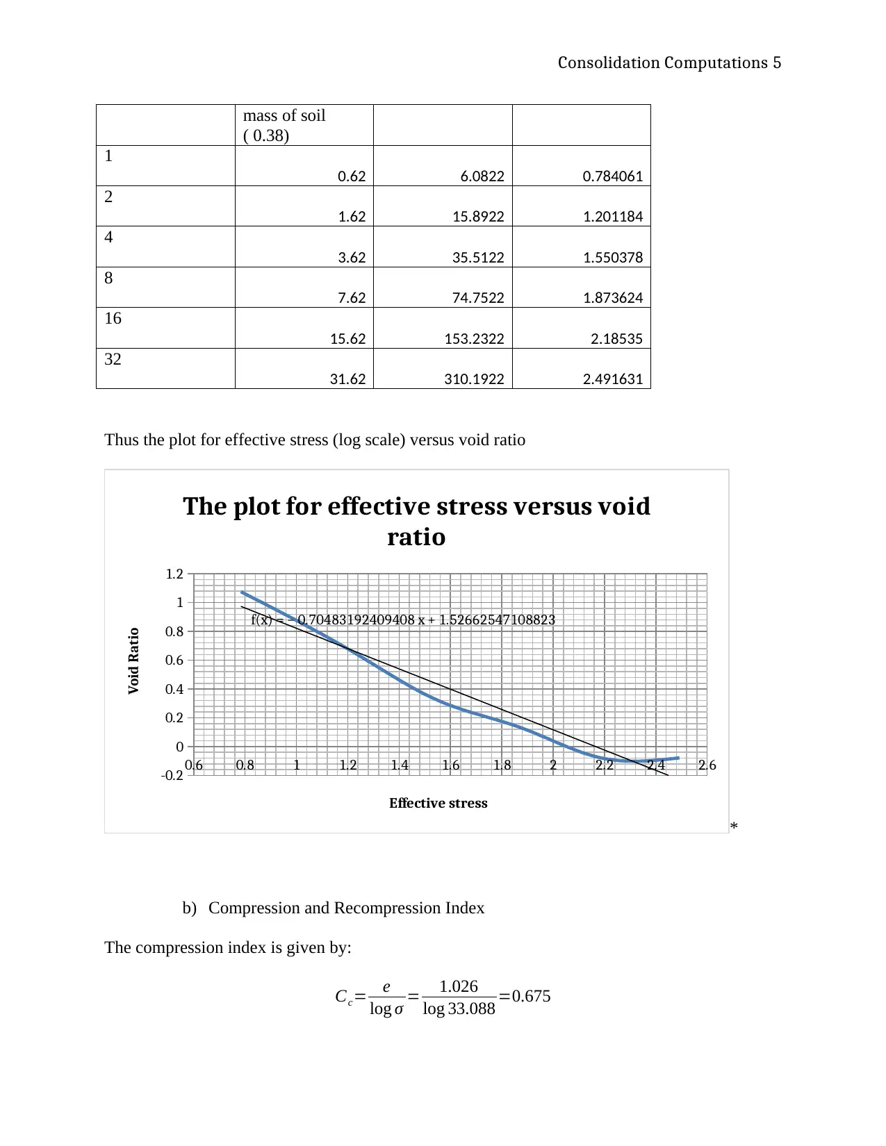
mass of soil
( 0.38)
1
0.62 6.0822 0.784061
2
1.62 15.8922 1.201184
4
3.62 35.5122 1.550378
8
7.62 74.7522 1.873624
16
15.62 153.2322 2.18535
32
31.62 310.1922 2.491631
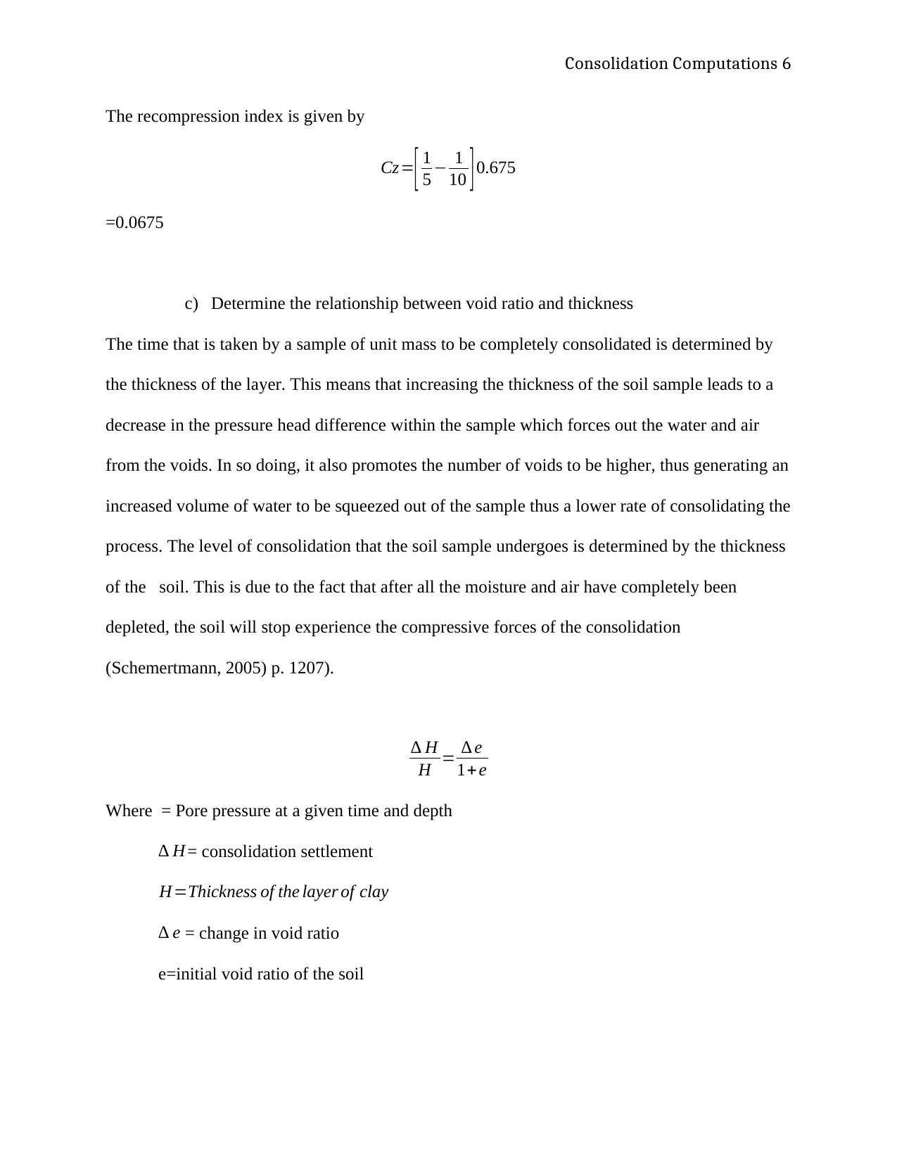
Thus the plot for effective stress (log scale) versus void ratio
0.6 0.8 1 1.2 1.4 1.6 1.8 2 2.2 2.4 2.6
-0.2
0
0.2
0.4
0.6
0.8
1
1.2
f(x) = − 0.70483192409408 x + 1.52662547108823
The plot for effective stress versus void
ratio
Effective stress
Void Ratio
*
b) Compression and Recompression Index
The compression index is given by:
Cc= e
log σ = 1.026
log 33.088 =0.675
mass of soil
( 0.38)
1
0.62 6.0822 0.784061
2
1.62 15.8922 1.201184
4
3.62 35.5122 1.550378
8
7.62 74.7522 1.873624
16
15.62 153.2322 2.18535
32
31.62 310.1922 2.491631
Thus the plot for effective stress (log scale) versus void ratio
0.6 0.8 1 1.2 1.4 1.6 1.8 2 2.2 2.4 2.6
-0.2
0
0.2
0.4
0.6
0.8
1
1.2
f(x) = − 0.70483192409408 x + 1.52662547108823
The plot for effective stress versus void
ratio
Effective stress
Void Ratio
*
b) Compression and Recompression Index
The compression index is given by:
Cc= e
log σ = 1.026
log 33.088 =0.675
Consolidation Computations 6
The recompression index is given by
Cz=
[ 1
5 − 1
10 ]0.675
=0.0675
c) Determine the relationship between void ratio and thickness
The time that is taken by a sample of unit mass to be completely consolidated is determined by
the thickness of the layer. This means that increasing the thickness of the soil sample leads to a
decrease in the pressure head difference within the sample which forces out the water and air
from the voids. In so doing, it also promotes the number of voids to be higher, thus generating an
increased volume of water to be squeezed out of the sample thus a lower rate of consolidating the
process. The level of consolidation that the soil sample undergoes is determined by the thickness
of the soil. This is due to the fact that after all the moisture and air have completely been
depleted, the soil will stop experience the compressive forces of the consolidation
(Schemertmann, 2005) p. 1207).
∆ H
H = ∆ e
1+ e
Where = Pore pressure at a given time and depth
∆ H = consolidation settlement
H=Thickness of the layer of clay=
∆ e = change in void ratio
e=initial void ratio of the soil
⊘ This is a preview!⊘
Do you want full access?
Subscribe today to unlock all pages.
Trusted by 1+ million students worldwide
Consolidation Computations 7
Pre-compression refers to the area of the loading before the planned structural is added to limit
settlement. It is also defined as the maximum effective over burden stress. It is also give by t
u=σ +σ '
u= [ h γ w− ( h+ y ) γsat ] −¿
u= [ ( 4∗9.81)− ( 4 +0.02 ) 18.041 ] −[4∗9.81+ ( 4 +0.02 ) 9.81]
u=33.088 kN /m3
(Burmeister, 2011)p. 83)
e) Co effiecient volume change between 200 and 800 Kpa effective stresses
T = Cv t
H2
33.088= 0.1968 Cv
0.01
Cv=2.802m2/year
2. Seepage Quantity
The layers of soil under the concrete mass are each 5m deep, meaning that they can be
considered as one anisotropic and homogenous soil layer of 10m thickness. The section is
transformed using a flownet as is shown in the figure below:
The coefficients of permeability of this homogenous layer of soil that is anisotropic in both the
vertical and horizontal directions is given by
Paraphrase This Document
Need a fresh take? Get an instant paraphrase of this document with our AI Paraphraser
Consolidation Computations 8
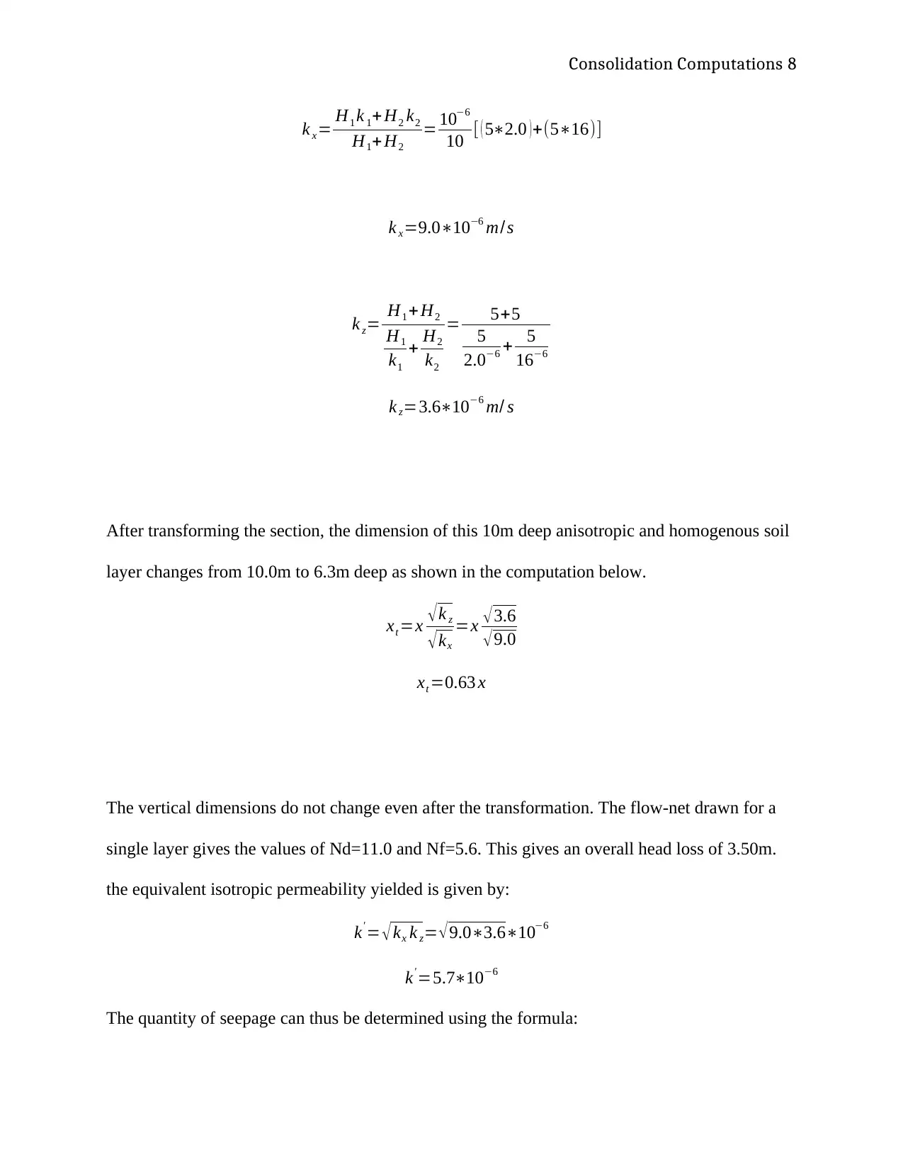
k x= H1 k 1+H2 k2
H1+H2
= 10−6
10 [ ( 5∗2.0 )+(5∗16)]
k x=9.0∗10−6 m/s
k z= H1 + H2
H1
k1
+ H2
k2
= 5+5
5
2.0−6 + 5
16−6
k z=3.6∗10−6 m/ s
After transforming the section, the dimension of this 10m deep anisotropic and homogenous soil
layer changes from 10.0m to 6.3m deep as shown in the computation below.
xt =x √k z
√kx
=x √3.6
√9.0
xt =0.63 x
The vertical dimensions do not change even after the transformation. The flow-net drawn for a
single layer gives the values of Nd=11.0 and Nf=5.6. This gives an overall head loss of 3.50m.
the equivalent isotropic permeability yielded is given by:
k' = √ kx k z= √9.0∗3.6∗10−6
k' =5.7∗10−6
The quantity of seepage can thus be determined using the formula:

Consolidation Computations 9
q=k ' h Nf
N d
=5.7∗10−6∗3.5∗5.6
11
q=1.0∗10−5 m3
s per meter
References
Burmeister, D., 2011. The application of controlled test methods in consolidation testing. ASTM
STP, 126(14), p. 83.
Schemertmann, J., 2005. The ndisturbed consolidation behavior of clay. Trans ASCE, 120(9), pp.
1201-1233.
q=k ' h Nf
N d
=5.7∗10−6∗3.5∗5.6
11
q=1.0∗10−5 m3
s per meter
References
Burmeister, D., 2011. The application of controlled test methods in consolidation testing. ASTM
STP, 126(14), p. 83.
Schemertmann, J., 2005. The ndisturbed consolidation behavior of clay. Trans ASCE, 120(9), pp.
1201-1233.
⊘ This is a preview!⊘
Do you want full access?
Subscribe today to unlock all pages.
Trusted by 1+ million students worldwide
1 out of 9
Your All-in-One AI-Powered Toolkit for Academic Success.
+13062052269
info@desklib.com
Available 24*7 on WhatsApp / Email
![[object Object]](/_next/static/media/star-bottom.7253800d.svg)
Unlock your academic potential
Copyright © 2020–2026 A2Z Services. All Rights Reserved. Developed and managed by ZUCOL.