Economics: Consumer Equilibrium, MRS, and Returns to Scale

This essay provides a comprehensive overview of three core economic concepts: consumer equilibrium, marginal rate of substitution (MRS), and returns to scale. The essay begins by defining consumer equilibrium, explaining how consumers maximize satisfaction within budget constraints, and differ...Read More

CONCEPTS ESSAY

Table of Contents
INTRODUCTION...........................................................................................................................3
MAIN BODY..................................................................................................................................3
ASSESSMENT 1.............................................................................................................................3
Consumer Equilibrium.................................................................................................................3
Marginal rate of Substitution.......................................................................................................5
Returns to Scale...........................................................................................................................7
CONCLUSION................................................................................................................................9
REFERENCES................................................................................................................................1
Figure 1: Consumer Equilibrium in Single Commodity..................................................................3
Figure 2: Two Commodity Case......................................................................................................4
Figure 3: Consumer Equilibrium in Two Commodity Case............................................................5
Figure 4: Indifference Curve and MRS...........................................................................................6
Figure 5: Different stages of return to scale....................................................................................7
Figure 6: Increasing returns to scale................................................................................................8
Figure 7: Constant returns to scale..................................................................................................8
Figure 8: Diminishing returns to scale.............................................................................................9

INTRODUCTION
In this report, a short essay has been presented on three different topics i.e. Consumer
Equilibrium, Marginal rate of substitution and Returns to scale.
MAIN BODY
ASSESSMENT 1
Consumer Equilibrium
Consumer Equilibrium can be defined as a situation in which the consumer has achieved
maximum level of satisfaction within a given income level and is in a state of balance without
any intended change in the current state (Ming and Tunca, 2019). There are two classification of
consumer equilibrium into single commodity and two commodities.
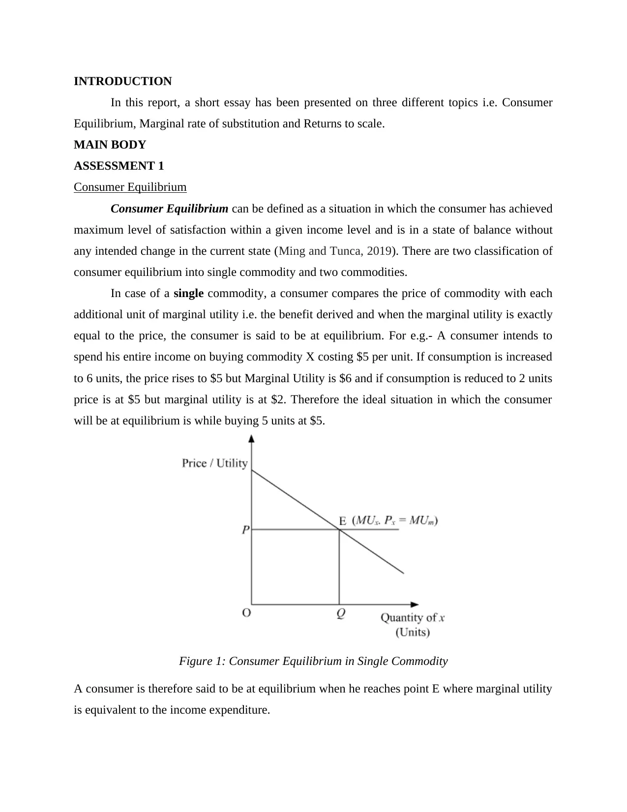
In case of a single commodity, a consumer compares the price of commodity with each
additional unit of marginal utility i.e. the benefit derived and when the marginal utility is exactly
equal to the price, the consumer is said to be at equilibrium. For e.g.- A consumer intends to
spend his entire income on buying commodity X costing $5 per unit. If consumption is increased
to 6 units, the price rises to $5 but Marginal Utility is $6 and if consumption is reduced to 2 units
price is at $5 but marginal utility is at $2. Therefore the ideal situation in which the consumer
will be at equilibrium is while buying 5 units at $5.
Figure 1: Consumer Equilibrium in Single Commodity
A consumer is therefore said to be at equilibrium when he reaches point E where marginal utility
is equivalent to the income expenditure.

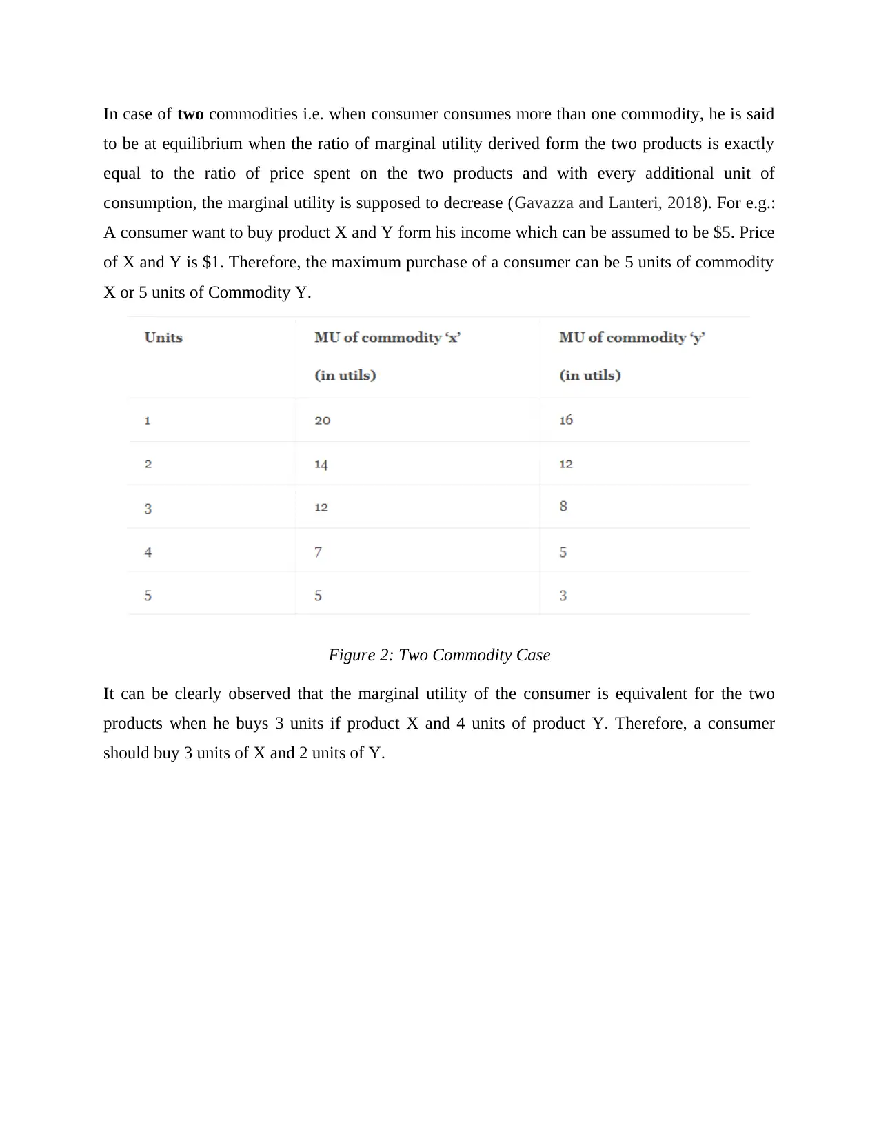
In case of two commodities i.e. when consumer consumes more than one commodity, he is said
to be at equilibrium when the ratio of marginal utility derived form the two products is exactly
equal to the ratio of price spent on the two products and with every additional unit of
consumption, the marginal utility is supposed to decrease (Gavazza and Lanteri, 2018). For e.g.:
A consumer want to buy product X and Y form his income which can be assumed to be $5. Price
of X and Y is $1. Therefore, the maximum purchase of a consumer can be 5 units of commodity
X or 5 units of Commodity Y.
Figure 2: Two Commodity Case
It can be clearly observed that the marginal utility of the consumer is equivalent for the two
products when he buys 3 units if product X and 4 units of product Y. Therefore, a consumer
should buy 3 units of X and 2 units of Y.

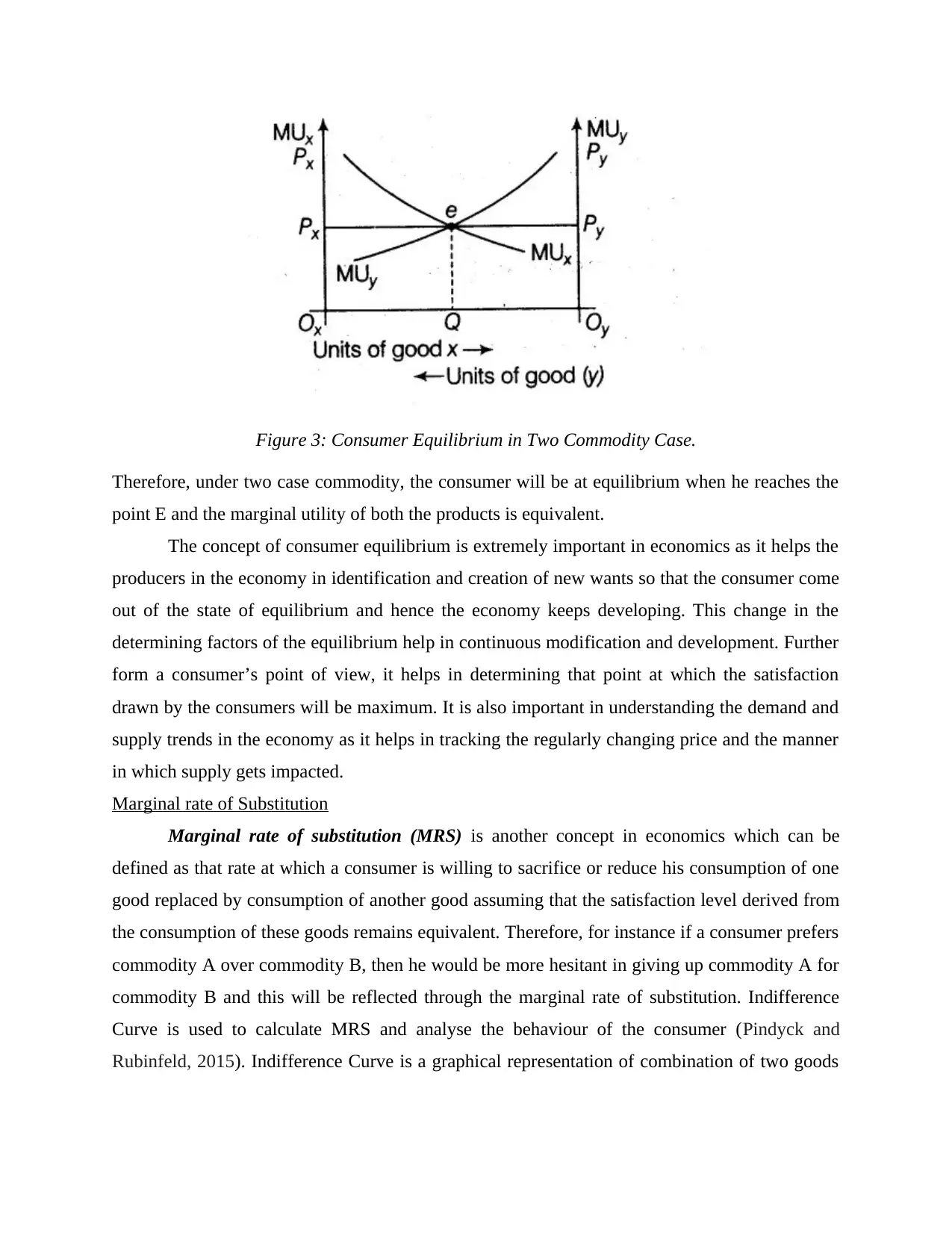
Figure 3: Consumer Equilibrium in Two Commodity Case.
Therefore, under two case commodity, the consumer will be at equilibrium when he reaches the
point E and the marginal utility of both the products is equivalent.
The concept of consumer equilibrium is extremely important in economics as it helps the
producers in the economy in identification and creation of new wants so that the consumer come
out of the state of equilibrium and hence the economy keeps developing. This change in the
determining factors of the equilibrium help in continuous modification and development. Further
form a consumer’s point of view, it helps in determining that point at which the satisfaction
drawn by the consumers will be maximum. It is also important in understanding the demand and
supply trends in the economy as it helps in tracking the regularly changing price and the manner
in which supply gets impacted.
Marginal rate of Substitution
Marginal rate of substitution (MRS) is another concept in economics which can be
defined as that rate at which a consumer is willing to sacrifice or reduce his consumption of one
good replaced by consumption of another good assuming that the satisfaction level derived from
the consumption of these goods remains equivalent. Therefore, for instance if a consumer prefers
commodity A over commodity B, then he would be more hesitant in giving up commodity A for
commodity B and this will be reflected through the marginal rate of substitution. Indifference
Curve is used to calculate MRS and analyse the behaviour of the consumer (Pindyck and
Rubinfeld, 2015). Indifference Curve is a graphical representation of combination of two goods

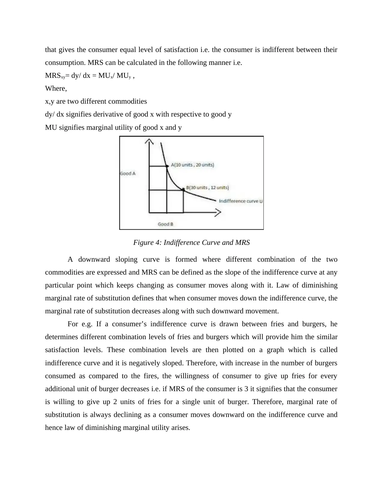
that gives the consumer equal level of satisfaction i.e. the consumer is indifferent between their
consumption. MRS can be calculated in the following manner i.e.
MRSxy= dy/ dx = MUx/ MUy ,
Where,
x,y are two different commodities
dy/ dx signifies derivative of good x with respective to good y
MU signifies marginal utility of good x and y
Figure 4: Indifference Curve and MRS
A downward sloping curve is formed where different combination of the two
commodities are expressed and MRS can be defined as the slope of the indifference curve at any
particular point which keeps changing as consumer moves along with it. Law of diminishing
marginal rate of substitution defines that when consumer moves down the indifference curve, the
marginal rate of substitution decreases along with such downward movement.
For e.g. If a consumer’s indifference curve is drawn between fries and burgers, he
determines different combination levels of fries and burgers which will provide him the similar
satisfaction levels. These combination levels are then plotted on a graph which is called
indifference curve and it is negatively sloped. Therefore, with increase in the number of burgers
consumed as compared to the fires, the willingness of consumer to give up fries for every
additional unit of burger decreases i.e. if MRS of the consumer is 3 it signifies that the consumer
is willing to give up 2 units of fries for a single unit of burger. Therefore, marginal rate of
substitution is always declining as a consumer moves downward on the indifference curve and
hence law of diminishing marginal utility arises.

Marginal Rate of Substitution helps in determining the indifference level of a consumer
for two products and helps the consumer in gaining maximum utility for a consumer within the
constraint of allocated budget (Berton and Migheli, 2015). It also helps in determining how much
value a single unit of particular commodity holds as compared to the value of multiple units of
another factors. When the concept of MRS is combined with budget constraint and its allocation,
the consumer is able to adopt most rational; allocation of its resources and utilize maximum
satisfaction. Therefore, the consumer will be able to utilize maximum benefit at certain points of
his indifference cycle.
Returns to Scale
Returns to scale is usually associated with the production aspect of a company in long run
i.e. all the inputs factors of production are treated as variables and can change with change in
scale or size. It illustrates the relationship between the input and output i.e. the rate at which the
production i.e. the output rises when the inputs of the production unit are increased in long run
(Banker and Zhang, 2016). There are three broad classification in the returns to scale i.e.
increasing returns to scale, constant returns to scale and diminishing returns to scale. When the
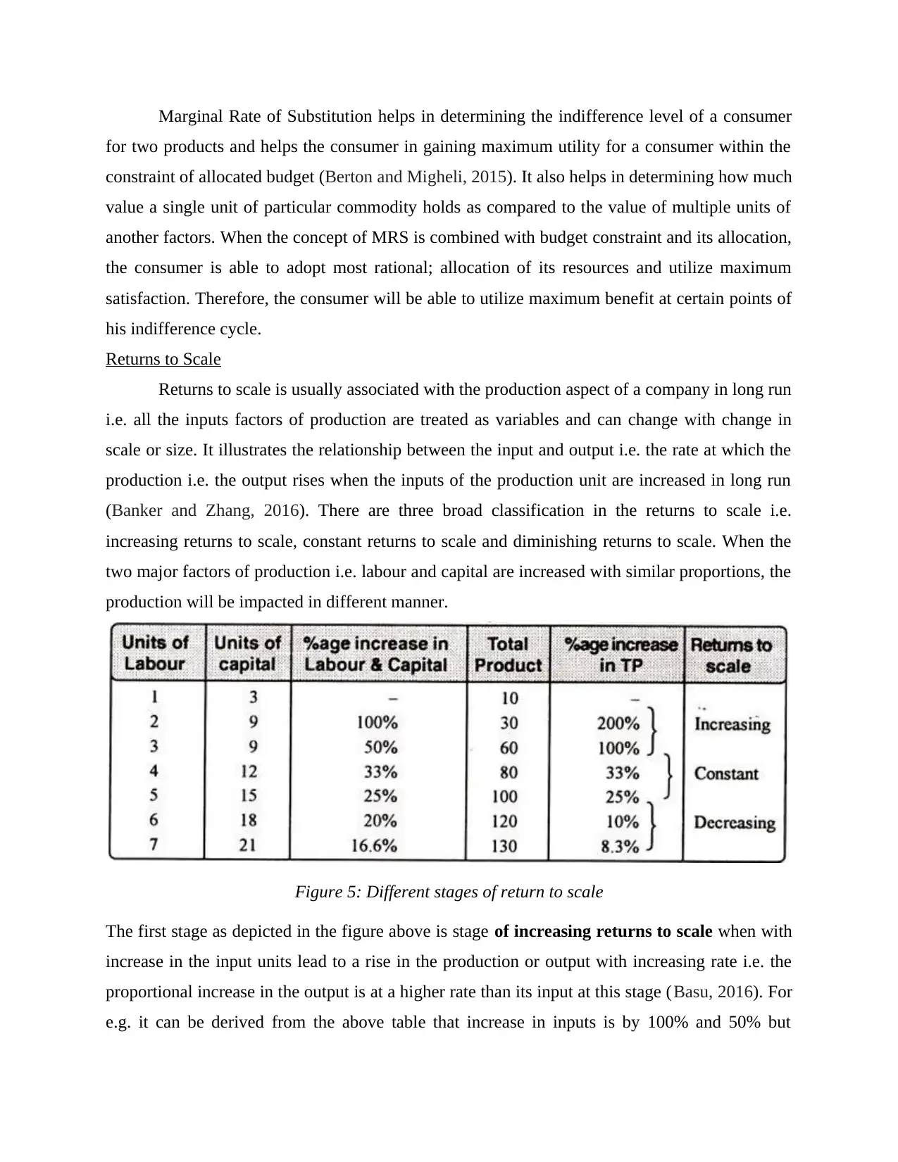
two major factors of production i.e. labour and capital are increased with similar proportions, the
production will be impacted in different manner.
Figure 5: Different stages of return to scale
The first stage as depicted in the figure above is stage of increasing returns to scale when with
increase in the input units lead to a rise in the production or output with increasing rate i.e. the
proportional increase in the output is at a higher rate than its input at this stage (Basu, 2016). For
e.g. it can be derived from the above table that increase in inputs is by 100% and 50% but

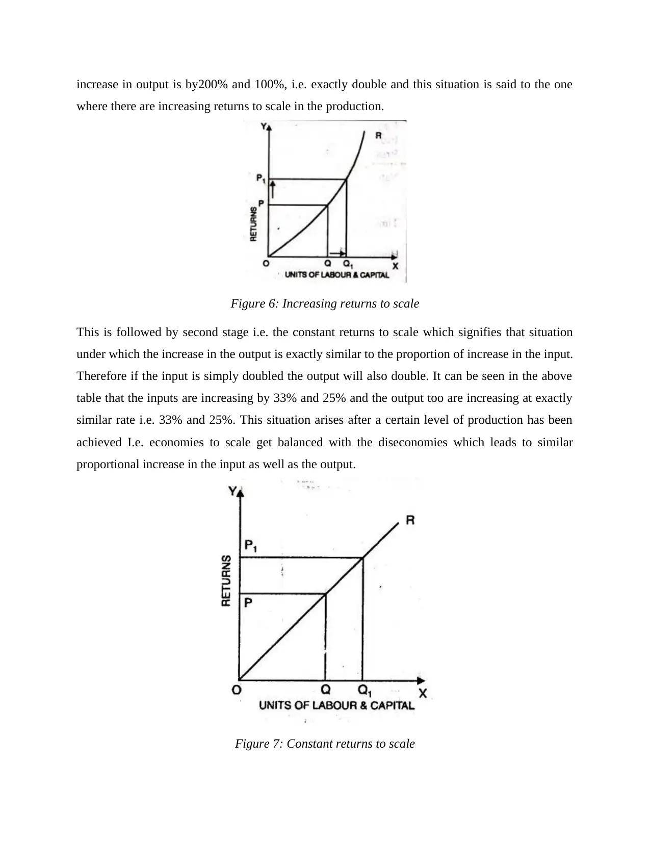
increase in output is by200% and 100%, i.e. exactly double and this situation is said to the one
where there are increasing returns to scale in the production.
Figure 6: Increasing returns to scale
This is followed by second stage i.e. the constant returns to scale which signifies that situation
under which the increase in the output is exactly similar to the proportion of increase in the input.
Therefore if the input is simply doubled the output will also double. It can be seen in the above
table that the inputs are increasing by 33% and 25% and the output too are increasing at exactly
similar rate i.e. 33% and 25%. This situation arises after a certain level of production has been
achieved I.e. economies to scale get balanced with the diseconomies which leads to similar
proportional increase in the input as well as the output.
Figure 7: Constant returns to scale

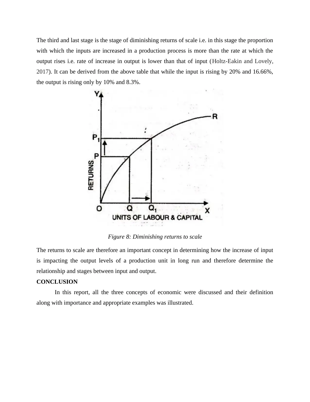
The third and last stage is the stage of diminishing returns of scale i.e. in this stage the proportion
with which the inputs are increased in a production process is more than the rate at which the
output rises i.e. rate of increase in output is lower than that of input (Holtz-Eakin and Lovely,
2017). It can be derived from the above table that while the input is rising by 20% and 16.66%,
the output is rising only by 10% and 8.3%.
Figure 8: Diminishing returns to scale
The returns to scale are therefore an important concept in determining how the increase of input
is impacting the output levels of a production unit in long run and therefore determine the
relationship and stages between input and output.
CONCLUSION
In this report, all the three concepts of economic were discussed and their definition
along with importance and appropriate examples was illustrated.

REFERENCES
Books and journals
Banker, R. and Zhang, D., 2016. The returns to scale assumption in incentive rate regulation.
Tech. rep., Temple University.
Basu, S., 2016. Returns to scale measurement. The New Palgrave Dictionary of Economics,
pp.1-5.
Berton, F. and Migheli, M., 2015. Estimating the marginal rate of substitution between wage and
employment protection.
Gavazza, A. and Lanteri, A., 2018. Credit shocks and equilibrium dynamics in consumer durable
goods markets. Economic Research Initiatives at Duke (ERID) Working Paper
Forthcoming.
Holtz-Eakin, D. and Lovely, M.E., 2017. Scale economies, returns to variety, and the
productivity of public infrastructure. In international economic integration and domestic
performance (pp. 73-91).
Ming, L. and Tunca, T.I., 2019. Consumer equilibrium, demand effects, and efficiency in group
buying. Demand Effects, and Efficiency in Group Buying (March 13, 2019).
Pindyck, R.S. and Rubinfeld, D.L., 2015. Microeconomics. Boston: Pearson,.
Online
[Online]. Available through: <>
1