Analysis of Aggregate Consumption Function Using Time Series Data
VerifiedAdded on 2020/12/09
|25
|4752
|354
Report
AI Summary
This report provides a comprehensive analysis of the aggregate consumption function using time series data, focusing on the Australian economy. It begins by creating a time series dataset from the Eurostat database, discussing the concepts of consumption functions, anticipations, serial correlation, and stationarity. The report details the process of estimating an aggregate consumption function, addressing non-stationarity by examining alterations in the data. Task 2 involves an in-depth analysis of the time series dataset and a survey of consumer finances, utilizing logarithmic models, debt-to-income ratios, and gender-specific regressions. The report also presents the results of weighted and non-weighted regressions and includes diagnostic checks. The analysis uses Stata for econometric modeling and statistical analysis, including histograms, scatter plots, and regression outputs. The report concludes with a summary of the findings and includes do-files for both tasks in the appendix.

Assessment
Paraphrase This Document
Need a fresh take? Get an instant paraphrase of this document with our AI Paraphraser
Table of Contents
INTRODUCTION...........................................................................................................................3
Task 1...............................................................................................................................................3
1. Creation of time series dataset to calculate aggregate consumption function.........................3
Anticipations...............................................................................................................................4
Serial correlation.........................................................................................................................4
Stationarity..................................................................................................................................5
Estimating an aggregate consumption function..........................................................................8
Task 2.............................................................................................................................................10
1 Analysis of time series dataset and survey of consumer finances.........................................10
Logarithmic model....................................................................................................................12
Debt-to-income ratio.................................................................................................................14
Gender-specific regressions or dummy variables.....................................................................15
Main specification.....................................................................................................................17
Diagnostic checks......................................................................................................................17
Including extra variables and interaction terms........................................................................18
CONCLUSION..............................................................................................................................19
Appendix........................................................................................................................................20
Do-file for Task 1......................................................................................................................20
Do-file for Task 2......................................................................................................................22
INTRODUCTION
Time series dataset refers to data points which are graphed with respect to time. It
basically includes series taken at consecutive distributed points in time. Therefore, it is a
succession of discrete-time data. Consumption function refers to functional relationship between
gross national income and total consumption (Anselin, 2013). This report deals with creation of
time series dataset so that overall consumption function can be evaluated. Furthermore, synthesis
of time series dataset is done and also analysis of dataset which is based on survey of finances of
consumers is provided.
Task 1
1. Creation of time series dataset to calculate aggregate consumption function.
Time series dataset refers to quantity that represent values which are taken by variable or
entity in certain time like year, quarter or month. This series occur when same standards are
canned on regular basis. Consumption function is defined as a economic formula which is used
to correspond relationship between overall consumption and gross national income.
In this report, country which is chosen is Australia. This report contains data which have
been used derived from Eurostat database. It is a database with around 4600 datasets which
comprises of approx 1.2 billion statistical data values. Eurostat is considered as exploit of
statistical collection of information. It contains data of every quarter for minimal gross
expendable income for household sector, their terminal consumption disbursement of households
and price index which was 2013=200 Data is obtained from Eurostat database which is
accessible at million units of currency. Therefore, consumer price index is used which is
available on OECD website of Australia. In that house price index which was obtained from
Eurostat for 2013=200. It is not similar to inflation but it is approximate value which has been
used for creation of dataset in real conditions (Anselin, Florax and Rey, 2013).
There is no data available with respect to Australia; therefore data which is utilized is
fluctuated across quarters. House price index (hpi) refers to measurements of fluctuation in
prices of residential houses in a form of percentage change from particular start date. For this
repeat-sales regression, simple moving average and hedonic regression can be used for
calculations. It will function as proxy for wealth which is on based two variables which will be
⊘ This is a preview!⊘
Do you want full access?
Subscribe today to unlock all pages.
Trusted by 1+ million students worldwide
used in regression. After this alterations are made with usage of Microsoft Excel and then this
file has been exported to Stata. In this time dimensions were fixed and different entities were
renamed. Furthermore, Moodle is used for assessment.
Anticipations
Some assumptions were taken for time series regression, so that unbiased estimators can
be calculated
stochastic process which relates with linearity in parameters;
{(xt1, xt2, …, xtk, yt) where t varies from 1 to n and follows linear model which
includes value from yt = O0 + O1xt1 + …+ Okxtk + ut where range of t in ut is between 1 to n
which denotes errors (this includes sequence of periods, different parameters) and k is a variable.
Independent variables are not constant as well as they are not perfect linear accumulation
of other independent variables which are present in sample which means that there is no
perfect co linearity.
Accepted value of error ut is zero for every t’s value, such that E(ut|X) = 0), where E
represents explanatory variables and value of t lies in between 1 to n.
Ordinary least squares (OLS) value will be similar to true parameters, when these
assumptions or anticipations are taken into consideration. This is known as theorem of
unbiasedness of OLS for particular time series regressions.
Serial correlation
In context of cross-section regression, vital anticipation which was taken considers that
different observations on e and y are not related with each other that is cov (yt, ys) = cov (et, es) =
0 for t s where t and s refer to different time periods (Asteriou and Hall, 2015). In this s and t
denotes unlike time periods. But as per our considerations, these anticipations will be doubtful to
cling to. Wealth, income and consumption expenditure which are interrelated as they change
steadily and not rapidly, these values will be dependent on previous values which were obtained
at another time period this means that they are correlated.
Paraphrase This Document
Need a fresh take? Get an instant paraphrase of this document with our AI Paraphraser
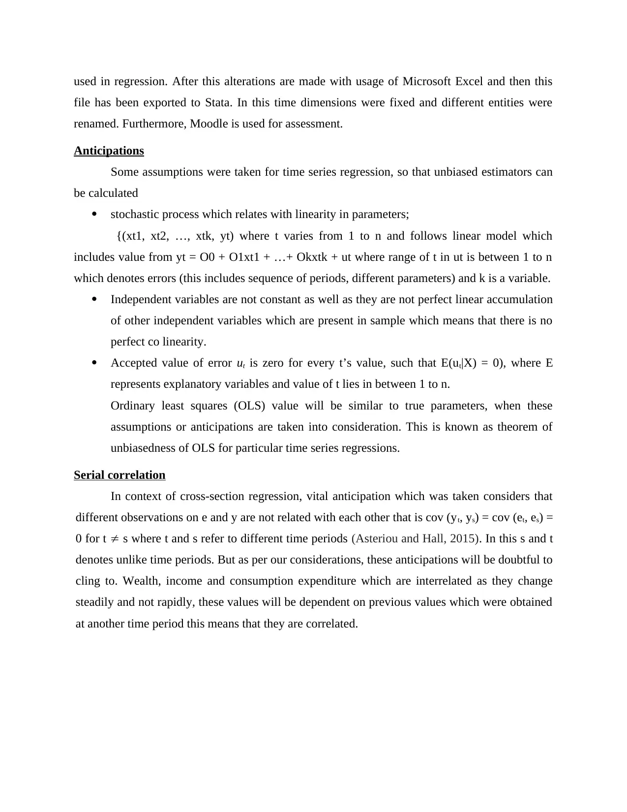
Figure 1 Autocorrelation of disposable income and expenditure consumption for ten different
lags.
In above figure, in both the cases for initial four autocorrelations are distinct from zero with 5%
level. When data is tested using Stata for autocorrelation then outcome obtained is clearer as it
can be seen in above figure. When taken into consideration, then it shows that disposable income
is dependent on previous disposable income (Brooks, 2019). These outcomes follow anticipation
for theorem of unbiasedness of OLS estimators for time series regression. It is not reliable to
depend on variance formula for estimator.
Stationarity
Anticipation is desecrated in dataset, therefore this section is taken into consideration.
From graphical representation it is clear that disposable income and consumption expenditure
will grow with time. Graphical representation will be in upward direction as it is already
mentioned above that Eurostat dataset is not adjusted seasonally rather than it is across quarter.
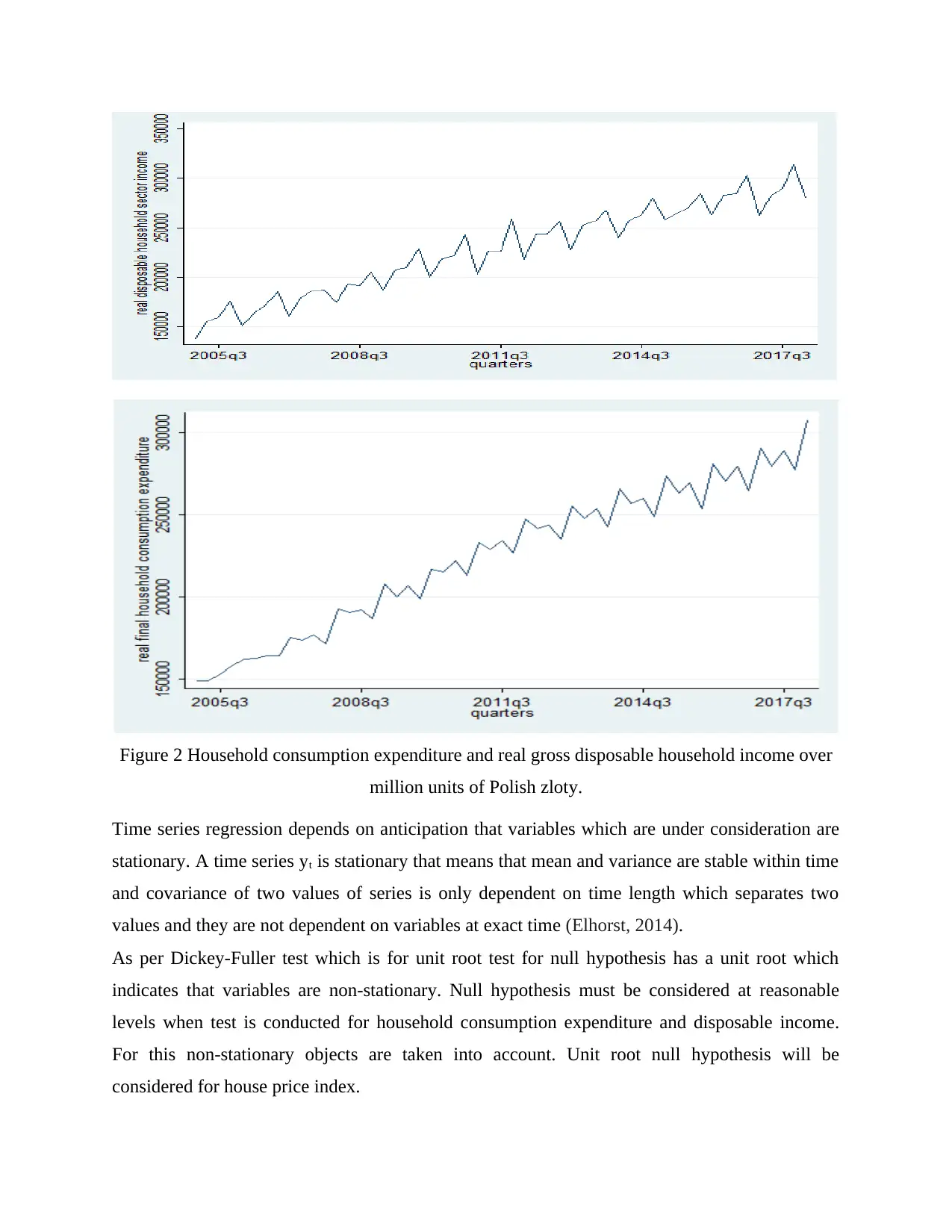
Figure 2 Household consumption expenditure and real gross disposable household income over
million units of Polish zloty.
Time series regression depends on anticipation that variables which are under consideration are
stationary. A time series yt is stationary that means that mean and variance are stable within time
and covariance of two values of series is only dependent on time length which separates two
values and they are not dependent on variables at exact time (Elhorst, 2014).
As per Dickey-Fuller test which is for unit root test for null hypothesis has a unit root which
indicates that variables are non-stationary. Null hypothesis must be considered at reasonable
levels when test is conducted for household consumption expenditure and disposable income.
For this non-stationary objects are taken into account. Unit root null hypothesis will be
considered for house price index.
⊘ This is a preview!⊘
Do you want full access?
Subscribe today to unlock all pages.
Trusted by 1+ million students worldwide
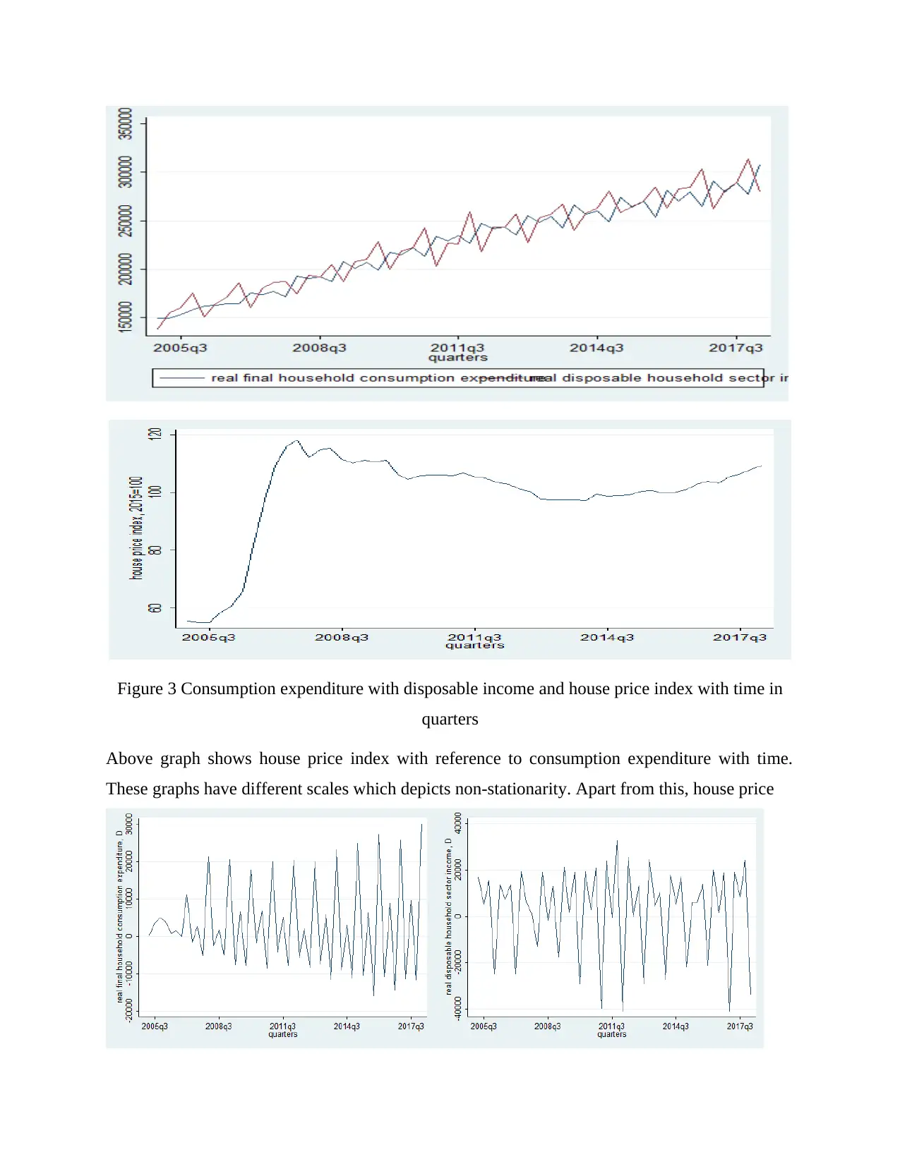
Figure 3 Consumption expenditure with disposable income and house price index with time in
quarters
Above graph shows house price index with reference to consumption expenditure with time.
These graphs have different scales which depicts non-stationarity. Apart from this, house price
quarters
Above graph shows house price index with reference to consumption expenditure with time.
These graphs have different scales which depicts non-stationarity. Apart from this, house price
Paraphrase This Document
Need a fresh take? Get an instant paraphrase of this document with our AI Paraphraser
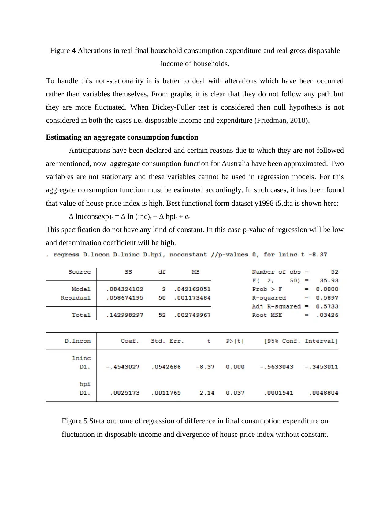
Figure 4 Alterations in real final household consumption expenditure and real gross disposable
income of households.
To handle this non-stationarity it is better to deal with alterations which have been occurred
rather than variables themselves. From graphs, it is clear that they do not follow any path but
they are more fluctuated. When Dickey-Fuller test is considered then null hypothesis is not
considered in both the cases i.e. disposable income and expenditure (Friedman, 2018).
Estimating an aggregate consumption function
Anticipations have been declared and certain reasons due to which they are not followed
are mentioned, now aggregate consumption function for Australia have been approximated. Two
variables are not stationary and these variables cannot be used in regression models. For this
aggregate consumption function must be estimated accordingly. In such cases, it has been found
that value of house price index is high. Best functional form dataset y1998 i5.dta is shown here:
∆ ln(consexp)t = ∆ ln (inc)t + ∆ hpit + et
This specification do not have any kind of constant. In this case p-value of regression will be low
and determination coefficient will be high.
Figure 5 Stata outcome of regression of difference in final consumption expenditure on
fluctuation in disposable income and divergence of house price index without constant.
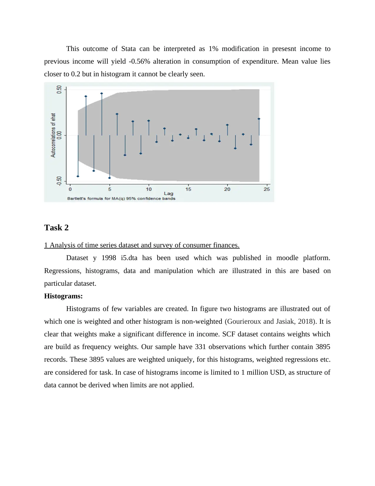
This outcome of Stata can be interpreted as 1% modification in presesnt income to
previous income will yield -0.56% alteration in consumption of expenditure. Mean value lies
closer to 0.2 but in histogram it cannot be clearly seen.
Task 2
1 Analysis of time series dataset and survey of consumer finances.
Dataset y 1998 i5.dta has been used which was published in moodle platform.
Regressions, histograms, data and manipulation which are illustrated in this are based on
particular dataset.
Histograms:
Histograms of few variables are created. In figure two histograms are illustrated out of
which one is weighted and other histogram is non-weighted (Gourieroux and Jasiak, 2018). It is
clear that weights make a significant difference in income. SCF dataset contains weights which
are build as frequency weights. Our sample have 331 observations which further contain 3895
records. These 3895 values are weighted uniquely, for this histograms, weighted regressions etc.
are considered for task. In case of histograms income is limited to 1 million USD, as structure of
data cannot be derived when limits are not applied.
⊘ This is a preview!⊘
Do you want full access?
Subscribe today to unlock all pages.
Trusted by 1+ million students worldwide
0 2 . 0 e - 0 64 . 0 e - 0 66 . 0 e - 0 68 . 0 e - 0 6
D e n s i t y
0 200000 400000 600000 800000 1000000
income
0 2 . 0 e - 0 64 . 0 e - 0 66 . 0 e - 0 68 . 0 e - 0 61 . 0 e - 0 5
D e n s i t y
0 200000 400000 600000 800000 1000000
income
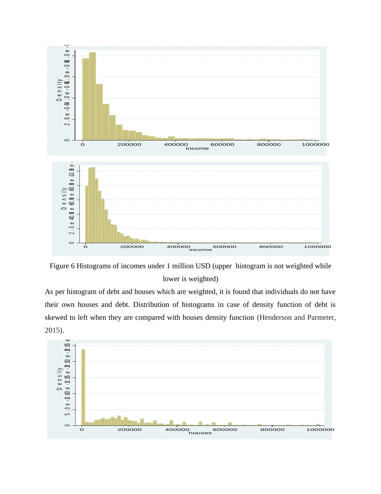
Figure 6 Histograms of incomes under 1 million USD (upper histogram is not weighted while
lower is weighted)
As per histogram of debt and houses which are weighted, it is found that individuals do not have
their own houses and debt. Distribution of histograms in case of density function of debt is
skewed to left when they are compared with houses density function (Henderson and Parmeter,
2015).
0 5 . 0 e - 0 61 . 0 e - 0 51 . 5 e - 0 52 . 0 e - 0 52 . 5 e - 0 5
D e n s i t y
0 200000 400000 600000 800000 1000000
houses
D e n s i t y
0 200000 400000 600000 800000 1000000
income
0 2 . 0 e - 0 64 . 0 e - 0 66 . 0 e - 0 68 . 0 e - 0 61 . 0 e - 0 5
D e n s i t y
0 200000 400000 600000 800000 1000000
income
Figure 6 Histograms of incomes under 1 million USD (upper histogram is not weighted while
lower is weighted)
As per histogram of debt and houses which are weighted, it is found that individuals do not have
their own houses and debt. Distribution of histograms in case of density function of debt is
skewed to left when they are compared with houses density function (Henderson and Parmeter,
2015).
0 5 . 0 e - 0 61 . 0 e - 0 51 . 5 e - 0 52 . 0 e - 0 52 . 5 e - 0 5
D e n s i t y
0 200000 400000 600000 800000 1000000
houses
Paraphrase This Document
Need a fresh take? Get an instant paraphrase of this document with our AI Paraphraser
0 1 . 0 e - 0 5 2 . 0 e - 0 5 3 . 0 e - 0 5
D e n s i t y
0 200000 400000 600000 800000 1000000
debt
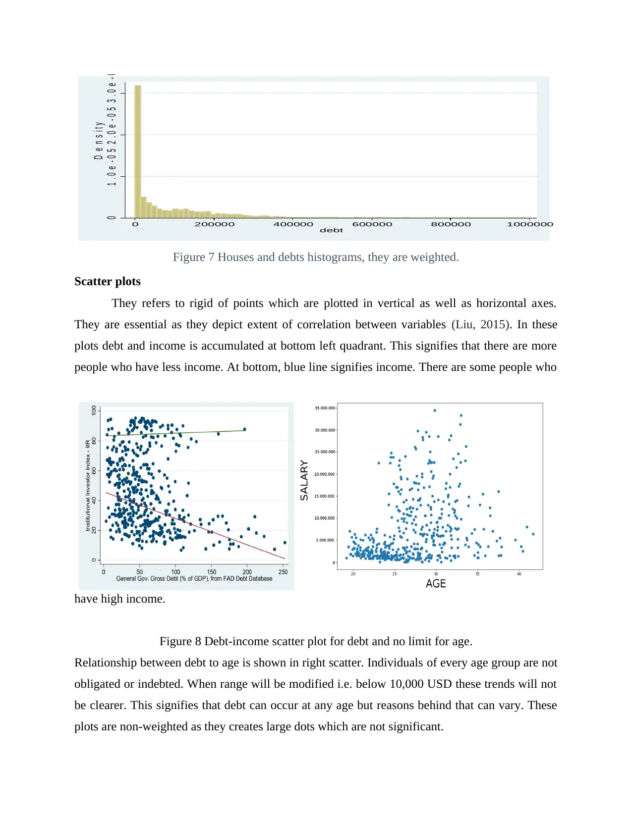
Figure 7 Houses and debts histograms, they are weighted.
Scatter plots
They refers to rigid of points which are plotted in vertical as well as horizontal axes.
They are essential as they depict extent of correlation between variables (Liu, 2015). In these
plots debt and income is accumulated at bottom left quadrant. This signifies that there are more
people who have less income. At bottom, blue line signifies income. There are some people who
have high income.
Figure 8 Debt-income scatter plot for debt and no limit for age.
Relationship between debt to age is shown in right scatter. Individuals of every age group are not
obligated or indebted. When range will be modified i.e. below 10,000 USD these trends will not
be clearer. This signifies that debt can occur at any age but reasons behind that can vary. These
plots are non-weighted as they creates large dots which are not significant.
D e n s i t y
0 200000 400000 600000 800000 1000000
debt
Figure 7 Houses and debts histograms, they are weighted.
Scatter plots
They refers to rigid of points which are plotted in vertical as well as horizontal axes.
They are essential as they depict extent of correlation between variables (Liu, 2015). In these
plots debt and income is accumulated at bottom left quadrant. This signifies that there are more
people who have less income. At bottom, blue line signifies income. There are some people who
have high income.
Figure 8 Debt-income scatter plot for debt and no limit for age.
Relationship between debt to age is shown in right scatter. Individuals of every age group are not
obligated or indebted. When range will be modified i.e. below 10,000 USD these trends will not
be clearer. This signifies that debt can occur at any age but reasons behind that can vary. These
plots are non-weighted as they creates large dots which are not significant.
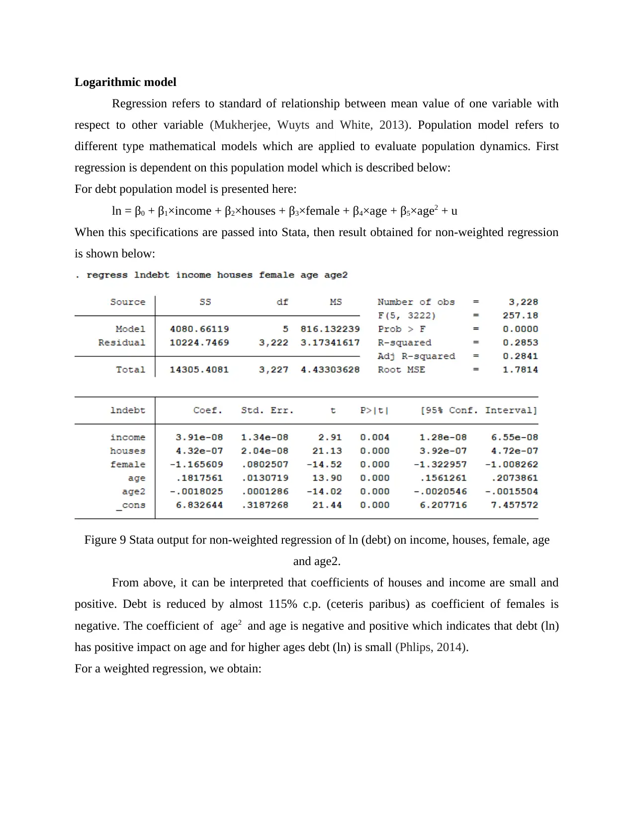
Logarithmic model
Regression refers to standard of relationship between mean value of one variable with
respect to other variable (Mukherjee, Wuyts and White, 2013). Population model refers to
different type mathematical models which are applied to evaluate population dynamics. First
regression is dependent on this population model which is described below:
For debt population model is presented here:
ln = β0 + β1×income + β2×houses + β3×female + β4×age + β5×age2 + u
When this specifications are passed into Stata, then result obtained for non-weighted regression
is shown below:
Figure 9 Stata output for non-weighted regression of ln (debt) on income, houses, female, age
and age2.
From above, it can be interpreted that coefficients of houses and income are small and
positive. Debt is reduced by almost 115% c.p. (ceteris paribus) as coefficient of females is
negative. The coefficient of age2 and age is negative and positive which indicates that debt (ln)
has positive impact on age and for higher ages debt (ln) is small (Phlips, 2014).
For a weighted regression, we obtain:
⊘ This is a preview!⊘
Do you want full access?
Subscribe today to unlock all pages.
Trusted by 1+ million students worldwide
1 out of 25

Your All-in-One AI-Powered Toolkit for Academic Success.
+13062052269
info@desklib.com
Available 24*7 on WhatsApp / Email
![[object Object]](/_next/static/media/star-bottom.7253800d.svg)
Unlock your academic potential
Copyright © 2020–2026 A2Z Services. All Rights Reserved. Developed and managed by ZUCOL.