Control Systems Assignment Solution: Stability and Controller Design

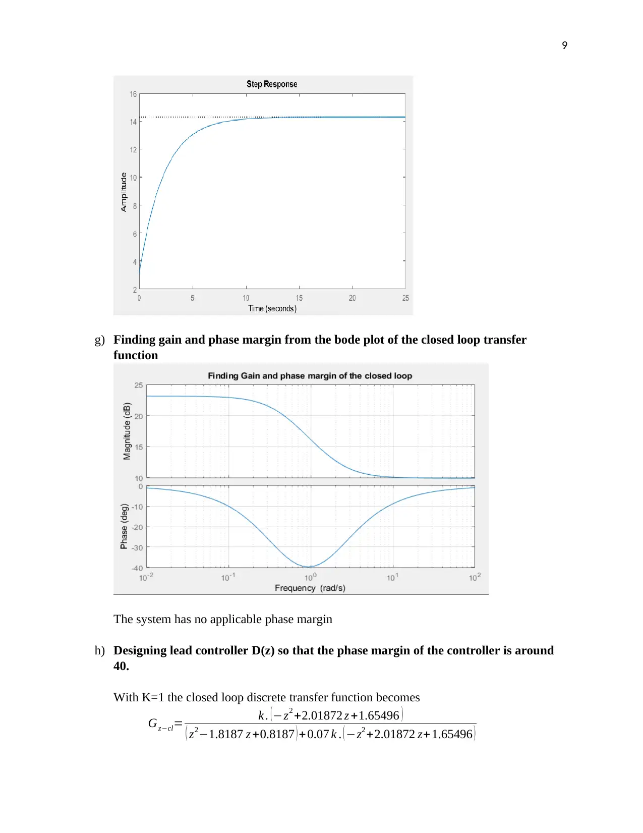
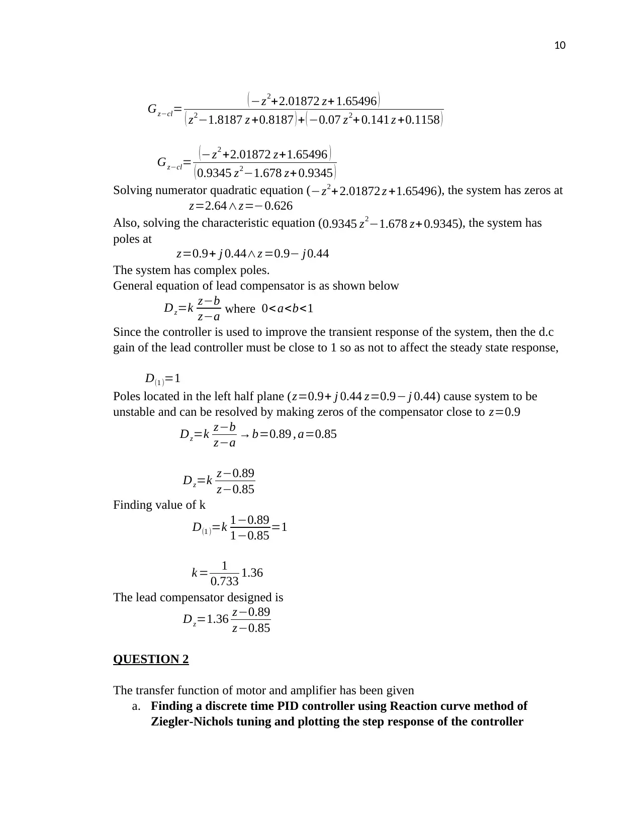
This document presents a detailed solution to a control systems assignment, encompassing several key aspects of control theory. The solution begins with an analysis of a robot arm control system, including the derivation of the closed-loop system characteristic equation and stability analysis using the Jury test. It then explores stability using the Nyquist and root locus methods, determining the range of gain (k) for stability. The assignment also covers the calculation of the steady-state error for a step response and the plotting of the closed-loop system's step response using Matlab. Furthermore, the solution includes the design of a lead controller to achieve a desired phase margin and the design of PID controllers using both the reaction curve and instability methods of Ziegler-Nichols tuning. The PID controllers are then discretized using backward and forward methods, and their step responses are compared to the continuous-time controllers. The analysis also includes the determination of gain and phase margins from the Bode plot of the closed-loop transfer function. The document provides Matlab code and Simulink diagrams to support the analysis and design processes, offering a comprehensive understanding of the concepts involved.

1
Student
Instructor
Control system
Date

2
QUESTION 1
The system below shows a robot arm control system. Assuming the sampling time Ts=0.1s and
assuming the digital controller transfer function is D(z)=1. Calculating the following
a) Writing the closed loop system characteristic equation.
Open loop transfer function
Gs =Ds × 200
s ( 0.5 s+1 ) × 1
100
Gs = 2
1
2 s ( s +2 )
= 4
s (s +2)
Converting to discrete transfer function with ZOH
Gz=( z−1
z )Z (Gs
s )= ( z−1
z )Z ( 1
s2 [ 4
s +2 ])
Z ( 1
s2 [ 4
s+2 ] )=Z ( 2
s2 − 1
s + 1
s+2 )
Z ( 2
s2 − 1
s + 1
s +2 )= [ 2t− y ( t )+ e−2 t ]
[ 2 t− y ( t ) +e−2 t ] =2 Tz
( z−1 ) 2 − z
z−1 + z
z−e−2 T
Gz=( z−1
z ) [ 2 0.1 z
( z−1 ) 2 − z
z−1 + z
z−0.8187 ]
Gz= [ 0.2
z−1 −1+ z (z−1)
z ( z−0.8187 ) ]
Gz= [ 0.2 ( z2−0.8187 z )− ( z2−0.8187 z ) ( z−1 ) +( z−1)(z2−z)
( z2 −0.8187 z ) ( z−1 ) ]
Gz= [ 2 z3 −3.6182 z2−0.98074 z +1
z3−1.8187 z2 +0.8187 z ]
Closed loop transfer function

3
Gz−cl= k . Gz
1+k . H .Gz
= k . Gz
1+0.7 k .Gz
Gz−cl=
k . [ 2 z3−3.6182 z2−0.98074 z+1
z3 −1.8187 z2 +0.8187 z ]
1+0.07 k . [ 2 z3−3.6182 z2−0.98074 z +1
z3−1.8187 z2+ 0.8187 z ]
Gz−cl= k . ( 2 z3−3.6182 z2 −0.98074 z+ 1 )
( z3−1.8187 z2 +0.8187 z ) +0.07 k . ( 2 z3−3.6182 z2−0.98074 z +1 )
Closed loop characteristic equation is given by
( z3−1.8187 z2 +0.8187 z ) +0.07 k . ( 2 z3 −3.6182 z2−0.98074 z +1 ) =0
( 1−0.14 k ) z3+ (1.8187+ 0.253 k ) z2 + ( 0.819−0.0686 k ) z +0.07 k =0
Where ao= ( 1−0.14 k ) , a1= ( 1.8187+ 0.253 k ) ,∧a2= ( 0.819−0.0686 k ) ,
a3=0.07 k
b) Using Jury test to find the range of gain k for stability
Since the characteristic equation is of the second order, then only 3 stability conditions
applies [1].
a) |a3|<a0
|( 0.141 k )|<|( 1−0.14 k )|
|( 0.281 k )|< 1
Thus k > 1
0.2 8 1
k > 3.559
b) P ( 1 )>0
( 1−0.14 k ) z3+ (1.8187+ 0.253 k ) z2 + ( 0.819−0.0686 k ) z +0.07 k >0

4
( 1−0.14 k ) + ( 1.8187+0.253 k )+ ( 0.819−0.0686 k ) +0.07 k >0
3.6377+ 0.114 k >0
k > −3.6377
0.114
k >−31.9
c) P (−1 ) <0 since n=3, an odd number
( 1−0.14 k ) z3+ (1.8187+ 0.253 k ) z2 + ( 0.819−0.0686 k ) z +0.07 k <0
− ( 1−0.14 k ) + ( 1.819+0.253 k )− ( 0.819−0.0686 k ) <0
( 0.4616 k )> 0
k > 0
Combining all ranges, then k is
0<k <3.559
c) Finding the range of k for stability using Nyquist method.
Letting the value of k=1, then finding time continuous transfer function of the system
Gs = 4
s(s+2) = 4
(s¿ ¿2+ 2 s)¿
Feedback H=0.07
Gscl
= Gs
1+ H . Gs ¿ ¿= 4
( s¿ ¿2+2 s)+0.07(4)= 4
( s ¿¿ 2+ 2 s+0.28)¿ ¿
Replacing s=jw
G( jω)= 4
(( jw )¿ ¿2+2 jw+0.28)= 4
((−ω)¿¿ 2+ 2 jω+0.28)¿ ¿
The characteristic equation is
c=(−ω ¿¿ 2+2 jω+0.28)¿
Equating imagery part of c to zero
2 jω=0→ ω=0
Finding the gain when ω=0

5
|G( j 0)|= 4
0.28 =14.29
Thus −1
k =−14.29
For stability, point (−1
k ) should not be encircled by Nyquist unit circle
−1
k ←14.29
k <0.07
The above condition should be when
k >0
Therefore, Nyquist range of k values for stability is
0< k <0.07
The matlab code below plots Nyquist when value of gain (k=0.07)
%COde that plots Nyquist with maximum value of k=0.07
clc
clear all
s=tf('s')
%---Designed k gain
k=0.07
%closed loop transfer function
G1=4k/(s^2+2*s+0.2)
%plotting Nyquist plot
nyquist(G1)
%End of the Program
Nyquist plot

6
d) Finding the range of k for stability using root locus method
Gs = k 4
s(s+2) = 4 k
( s¿ ¿2+ 2 s)¿
From the closed loop transfer function
Gscl
= Gs
1+ H . k . Gs ¿ ¿= 4 k
(s¿¿ 2+2 s +0.28 k ) ¿
The system has poles at
p= {−0.15∧−1.85 }
No zeros are in the system
The characteristic equation is given by;
C=(s ¿¿ 2+ 2 s+0.28 k) ¿
Letting
0.28 k =0
Then for stability, the range of k should be
k >0
Matlab code for Rlocus method
%COde that plots rootlocus with minimum value of k>0=0.0009
clc
clear all

7
s=tf('s')
%---Designed k gain
k=0.0009
%closed loop transfer function
G1=4*k/(s^2+2*s+0.2)
%plotting rlocus plot
rlocus(G1)
%End of the Program
All poles are to the negative half plane, thus the system is stable.
e) Finding the state error of the closed loop system to a step response when k=1.
Gscl
= Gs
1+ H . k . Gs ¿ ¿= 4
( s¿¿ 2+2 s +0.28)¿
Finding state steady error for step input
ess=Limit
s →0 s Es
Where
Es= Rs
1+Gs H
Therefore

8
ess=Limit
s →0 s Rs
1+Gs H =s
1
s
¿ ¿
ess=Limit
s →0 s Rs
1+Gs H =(s¿¿ 2+2 s +0.28)
¿ ¿ ¿
ess=0.065
f) Plotting step response of the closed loop system in Matlab Simulink
This plot was implemented using Matlab Code script.

9
g) Finding gain and phase margin from the bode plot of the closed loop transfer
function
The system has no applicable phase margin
h) Designing lead controller D(z) so that the phase margin of the controller is around
40.
With K=1 the closed loop discrete transfer function becomes
Gz−cl= k . (−z2 +2.01872 z +1.65496 )
( z2−1.8187 z +0.8187 ) + 0.07 k . ( −z2 +2.01872 z+ 1.65496 )

10
Gz−cl= ( −z2+2.01872 z+ 1.65496 )
( z2−1.8187 z +0.8187 ) + ( −0.07 z2+0.141 z +0.1158 )
Gz−cl= (−z2 +2.01872 z+1.65496 )
(0.9345 z2−1.678 z+ 0.9345 )
Solving numerator quadratic equation (−z2+ 2.01872 z +1.65496), the system has zeros at
z=2.64∧z=−0.626
Also, solving the characteristic equation ( 0.9345 z2−1.678 z+ 0.9345), the system has
poles at
z=0.9+ j 0.44∧z =0.9− j0.44
The system has complex poles.
General equation of lead compensator is as shown below
Dz=k z−b
z−a where 0< a<b<1
Since the controller is used to improve the transient response of the system, then the d.c
gain of the lead controller must be close to 1 so as not to affect the steady state response,
D(1 )=1
Poles located in the left half plane ( z=0.9+ j 0.44 z=0.9− j 0.44) cause system to be
unstable and can be resolved by making zeros of the compensator close to z=0.9
Dz=k z−b
z−a →b=0.89 , a=0.85
Dz=k z−0.89
z−0.85
Finding value of k
D(1 )=k 1−0.89
1−0.85 =1
k = 1
0.733 1.36
The lead compensator designed is
Dz=1.36 z−0.89
z−0.85
QUESTION 2
The transfer function of motor and amplifier has been given
a. Finding a discrete time PID controller using Reaction curve method of
Ziegler-Nichols tuning and plotting the step response of the controller

11
Gp ( s )= 20
(s+ 1)(s+5) and GA ( s )= 0.5
(2 s+ 1)
Finding the combined closed loop system characteristic equation
C=1+Gp ( s ) GA (s ) (Kc)
Where ( Kc ) is thecontroller
C=1+ [ 20
( s +1 ) ( s+ 5 ) ][ 0.5
( 2 s +1 ) ] ( K c ) =0
C= 10(K c)
2 s3 +13 s2 +16 s +5 +1=0
C=2 s3+13 s2+16 s+5+10 KCU =0
Substituting s=jw
C=2( jω)3 +13( jω)2 +16( jω)+5+10 ¿
−2 j ω3 −13 ω2 +16( jω)+(5+10 KCU )=0
Finding w by solving imagery part
−2 j ω3 +16 ( jω )=0
ω= √ 16
2 = √ 8
Finding ultimate period time
Pu= 2 π
ω = 2 π
√8 =2.22
Finding gain Kcu by solving real part
−13 ω2+5+10 KCU =0
−13 ( 8 ) +5+10 KCU =0
10 Kc=99 → KCU=9.9
From Zieglar PID tuning table
Kp τ I τ d
PID KCU
1.7
PU
2
PU
8

12
5.62 1.11 0.2775
Time continuous PID controller designed
PID=k p (1+ τ I
s + τd s )=5.62 (1+ 1.11
s +0.2775 s )
The following Matlab code converts PID controller into digital form and plots step response of
the system
%BEGINNING OF THE CODE
clc
clear all
s=tf('s');
%Transfer function of the motor
Gp=20/((s+1)*(s+5))
%Transfer function of the amplifier
Ga=0.5/(2*s+1);
%Open loop transfer function
Gss=Ga*Gp;
%Designed constants of PID controller using reaction curve Ziegler
%--Nichols tuning
kp=5.94;
ti=5.35;
td=1.65;
%--Transfer function of the designed PID
PID=kp*(1+ti/s+td*s)
%Conversion to Dicrete
Ts=0.002 % Sampling period
PIDz=c2d(PID,Ts,'tustin')
%CLosed loop transfer function of the system
Gf=feedback(Gss*PID,1);
%Step response of the closed loop system
step(Gf)
stepinfo(Gf)
%END OF THE CODE
Digitized PID is
PIDd = 9807 z2 −1.96e04 z+ 9795
z2−1
Step response of the closed loop