Control Systems Homework Assignment Solution and Response Analysis
VerifiedAdded on 2022/08/22
|13
|791
|25
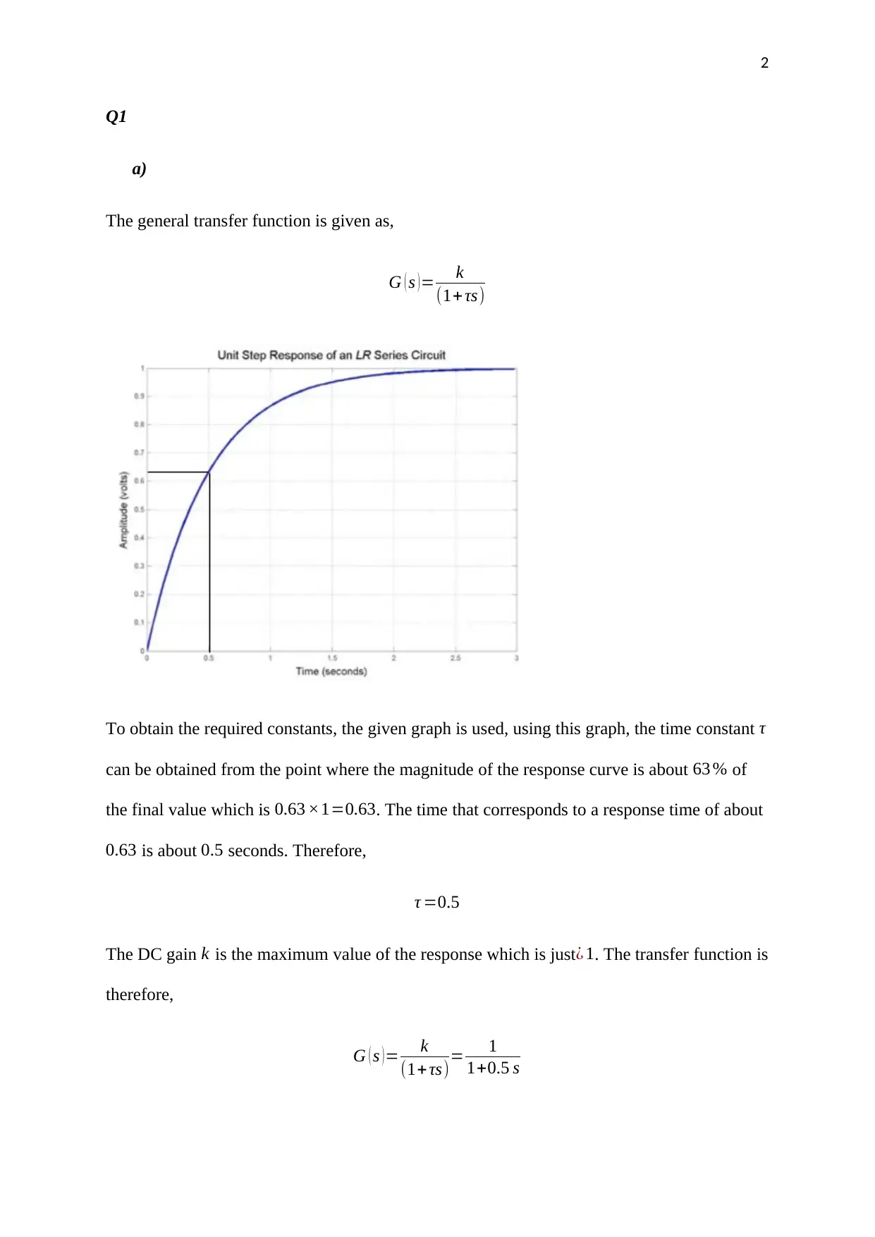
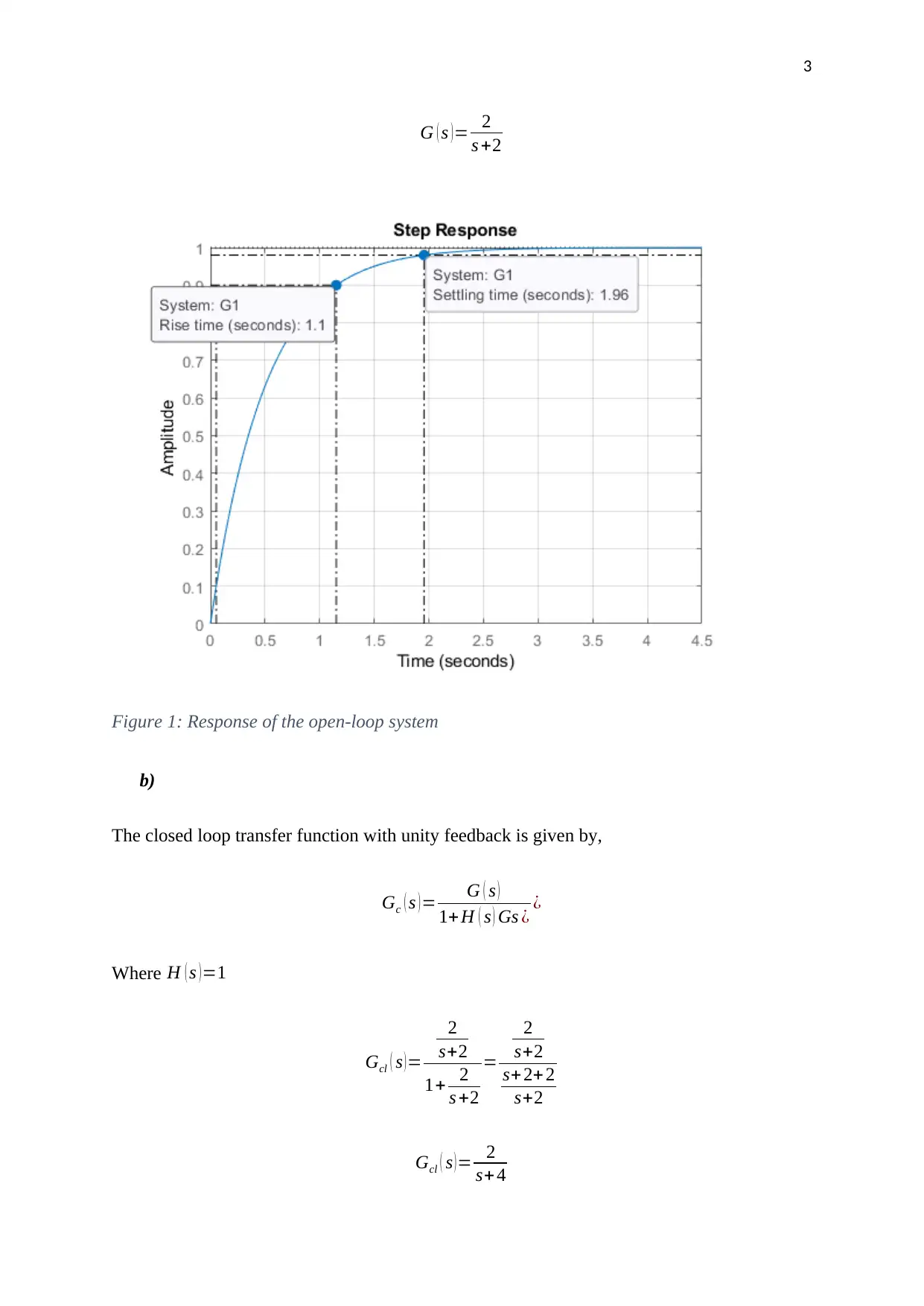
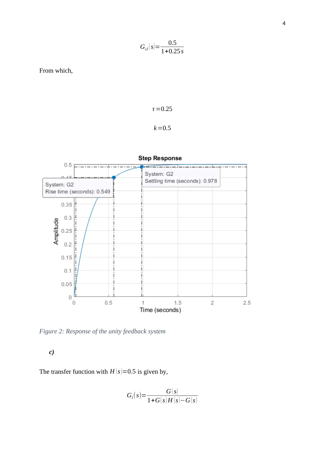
Homework Assignment
AI Summary
This document presents a complete solution to a control systems homework assignment, analyzing two different problems. The first problem focuses on determining the transfer function of an open-loop system and then analyzing the response of both unity and non-unity feedback systems. The solution involves deriving the transfer functions, calculating time constants, and comparing the transient responses of each system, including rise time and settling time. The second problem delves into a second-order system, deriving the transfer function from a given response graph. It calculates key parameters such as natural frequency and damping ratio. Furthermore, the solution compares the performance of open-loop, unity feedback, and non-unity feedback systems, including their stability and transient response characteristics. The document includes relevant graphs illustrating system responses and concludes with a bibliography of cited sources.

1 out of 13
Related Documents


Your All-in-One AI-Powered Toolkit for Academic Success.
+13062052269
info@desklib.com
Available 24*7 on WhatsApp / Email
![[object Object]](/_next/static/media/star-bottom.7253800d.svg)
Copyright © 2020–2026 A2Z Services. All Rights Reserved. Developed and managed by ZUCOL.