EEE 303A: Comprehensive Solutions for Control Systems Test 1 Problems

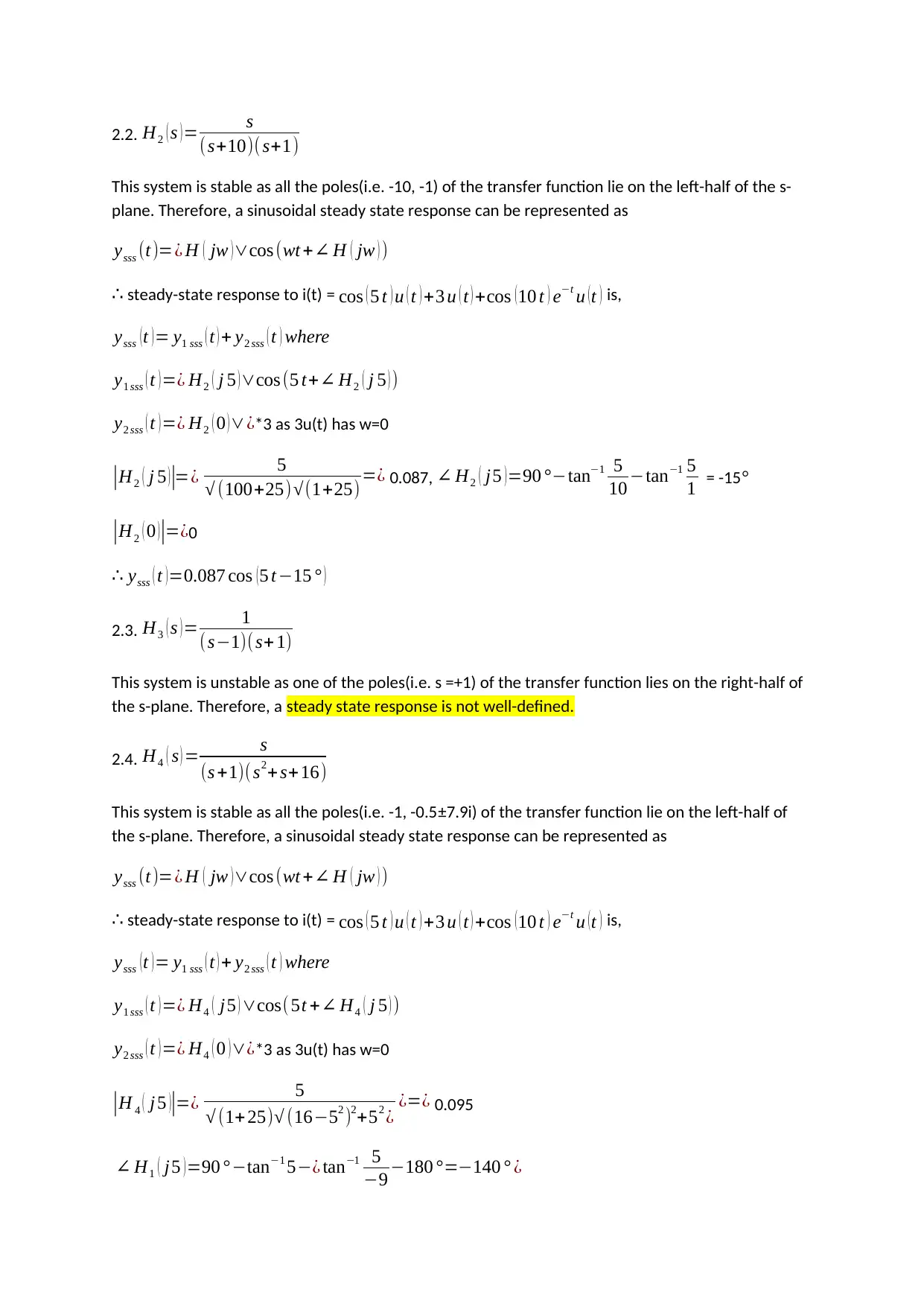
This document presents comprehensive solutions to an Electrical Engineering assignment, specifically focusing on control systems. The solutions cover various aspects, including the analysis of Continuous-Time (CT) and Discrete-Time (DT) systems. The assignment requires students to derive magnitude and phase expressions for Bode plots, sketch their asymptotes, and verify them using MATLAB. Furthermore, it involves computing the steady-state response of systems to given inputs, analyzing system stability, and designing a second-order high-pass Butterworth CT filter to remove slow drift from an AC signal. The solutions provide detailed step-by-step explanations, MATLAB code snippets, and graphical representations to aid in understanding the concepts and problem-solving techniques. The document addresses the critical aspects of control systems, providing valuable insights and practical examples for students to enhance their understanding of the subject.

SOLUTIONS: EEE 303A TEST1
Solution 1
Part-1
1.1. H1 ( s ) = ( s+1)
(s+2)( s2 + s+16)
Putting s = jw, we get
H1 ( jw ) = ( jw+ 1)
( jw+ 2)(−w2 + jw +16)
So, magnitude = |H1 ( jw )∨¿ √ (w2+1)
√ (w2+4)√ ((16−w2)+ w2 )
Phase = ∠ H1 ( jw ) =tan−1 w−tan−1 w
2 −¿ tan−1 w
(16−w2) −πu(w2−16)¿
Asymptotic plot:
Asymptotes at corner frequencies of 1 rad/s(20dB/dec, 90deg), 2 rad/s (-20dB/dec, -90deg) and √16
rad/s(-40dB/dec, -180deg)
The transfer function has quadratic terms in the denominator. On comparing the quadratic terms
with the standard form of s2 +2 ξ wn s+ wn
2, we get wn=¿ √16 and ξ= 1
8 =0.125<1. Hence, the
system is underdamped. The asymptotic plot also shows significant resonance.

Bode Plot: is generated using following MATLAB commands.
>>syms s
>>H=tf([1,1],[1,3,18,32])
>>bode(H)

1.2. H2 ( s )= s
(s+10)( s+1)
Putting s = jw, we get
H2 ( jw )= jw
( jw+ 10)( jw +1)
So, magnitude = | H2 ( jw ) ∨¿ w
√ (w2+100)√ (w2+1)
Phase = ∠ H2 ( jw ) = π
2 −tan−1 w
10 −¿ tan−1 w ¿
Asymptotic Plot:
Asymptotes at corner frequencies of 1rad/s (-20dB/dec, -90deg), 10rad/s (-20dB/dec, -90deg) and 0
rad/s(20dB/dec, 90deg)
Bode Plot: is generated using following MATLAB commands.
>>syms s

>>H=tf([1,0],[1,11,10])
>>bode(H)
1.3. H3 ( s )= 1
(s−1)( s+ 1)
Putting s = jw, we get
H3 ( jw )= 1
( jw−1)( jw +1)
So, magnitude = |H3 ( jw )∨¿ 1
(1+ w2)
Phase = ∠ H3 ( jw )=¿-π+tan−1 w
1 −¿ tan−1 w
1 ¿ = -π
Asymptotic Plot:
Asymptote at corner frequency of 1rad/s(-40dB/dec, -180deg)

Bode Plot: is generated using following MATLAB commands.
>>syms s
>>H=tf([1],[1,0,-1])
>>bode(H)

1.4. H4 ( s ) = s
(s +1)( s2+ s+16)
Putting s = jw, we get
H4 ( jw ) = jw
( jw +1)(−w2+ jw +16)
So, magnitude = | H4 ( jw ) ∨¿ w
√(w2 +1)√ ((16−w2)+w2)
Phase = ∠ H4 ( jw ) = π
2 −tan−1 w
1 −¿ tan−1 w
( 16−w2 )−πu (w2−16)¿
Asymptotic Plot:
Asymptotes at corner frequencies of 0 rad/s (+20dB/dec, +90deg), 1rad/s (-20dB/dec, -90deg) and
√16 rad/s(-40dB/dec, -180deg)
The transfer function has quadratic terms in the denominator. On comparing the quadratic terms
with the standard form of s2 +2 ξ wn s+ wn
2, we get wn=¿ √16 and ξ= 1
8 =0.125<1. Hence, the
system is underdamped. The asymptotic plot also shows significant resonance.

Bode Plot: is generated using following MATLAB commands.
>>syms s
>>H=tf([1,0],[1,2,17,16])
>>bode(H)

Part-2
2.1. H1 ( s )= ( s+1)
(s+2)( s2 + s+16)
This system is stable as all the poles(i.e. -2, -0.5±7.9i) of the transfer function lie on the left-half of
the s-plane. Therefore, a sinusoidal steady state response can be represented as
ysss (t)=¿ H ( jw ) ∨cos (wt +∠ H ( jw ) )
∴ steady-state response to i(t) = cos ( 5 t ) u ( t ) +3 u ( t ) +cos (10 t ) e−t u (t ) is,
ysss (t )= y1 sss ( t ) + y2 sss ( t ) where
y1 sss ( t ) =¿ H1 ( j 5 ) ∨cos (5 t+∠ H1 ( j 5 ) )
y2 sss ( t ) =¿ H1 ( 0 ) ∨¿*3 as 3u(t) has w=0
|H1 ( j 5 )|=¿ √ (1+ 25)
√ (4 +25)√(16−52 )2+52 ¿ ¿=¿ 0.09
∠ H1 ( j5 )=tan−1 5−tan−1 5
2 −¿ tan−1 5
−9 −180 °=−¿ ¿ 140.5°
|H1 ( 0 )|=¿1/32
∴ ysss ( t ) =0.09 cos ( 5 t −140.5 ° ) +3/32
The Third exponentially-decaying term is ignored as it gives transient response and finally, decays
with time.

2.2. H2 ( s )= s
(s+10)( s+1)
This system is stable as all the poles(i.e. -10, -1) of the transfer function lie on the left-half of the s-
plane. Therefore, a sinusoidal steady state response can be represented as
ysss (t)=¿ H ( jw ) ∨cos (wt +∠ H ( jw ) )
∴ steady-state response to i(t) = cos ( 5 t ) u ( t ) +3 u ( t ) +cos (10 t ) e−t u (t ) is,
ysss ( t ) = y1 sss ( t ) + y2 sss ( t ) where
y1 sss ( t )=¿ H2 ( j 5 )∨cos (5 t+∠ H2 ( j 5 ) )
y2 sss ( t ) =¿ H2 ( 0 ) ∨¿*3 as 3u(t) has w=0
|H2 ( j 5 )|=¿ 5
√ (100+25)√(1+25)=¿ 0.087, ∠ H2 ( j5 ) =90 °−tan−1 5
10 −tan−1 5
1 = -15°
|H2 ( 0 )|=¿0
∴ ysss ( t ) =0.087 cos ( 5 t−15 ° )
2.3. H3 ( s )= 1
(s−1)( s+ 1)
This system is unstable as one of the poles(i.e. s =+1) of the transfer function lies on the right-half of
the s-plane. Therefore, a steady state response is not well-defined.
2.4. H4 ( s ) = s
(s +1)( s2+ s+16)
This system is stable as all the poles(i.e. -1, -0.5±7.9i) of the transfer function lie on the left-half of
the s-plane. Therefore, a sinusoidal steady state response can be represented as
ysss (t)=¿ H ( jw ) ∨cos (wt +∠ H ( jw ) )
∴ steady-state response to i(t) = cos ( 5 t ) u ( t ) +3 u ( t ) +cos (10 t ) e−t u (t ) is,
ysss (t )= y1 sss ( t ) + y2 sss ( t ) where
y1 sss ( t ) =¿ H4 ( j5 ) ∨cos( 5t +∠ H4 ( j 5 ) )
y2 sss ( t )=¿ H4 ( 0 )∨¿*3 as 3u(t) has w=0
|H 4 ( j 5 )|=¿ 5
√ (1+ 25)√ (16−52 )2+52 ¿ ¿=¿ 0.095
∠ H1 ( j5 ) =90 ° −tan−1 5−¿ tan−1 5
−9 −180 °=−140 ° ¿

|H 4 ( 0 )|=¿0
∴ ysss ( t ) =0.095 cos ( 5 t−140 ° )
Solution 2
Part-1
1.1. H1 ( z ) = z
(z−0.5)( z−0.7)
Putting z = e j Ω, we get
H1 ( e j Ω ) = e j Ω
(e j Ω −0.5)(e j Ω −0.7) = cos Ω+ jsinΩ
(cos Ω−.5+ jsinΩ)(cos Ω−.7+ jsinΩ)
So, magnitude = | H1 ( e j Ω ) ∨¿ 1
√ (cos Ω−.5)2 +(sinΩ)2
√ (cos Ω−.7)2+(sinΩ)2
Phase = ∠ H1 ( e j Ω ) =Ω−tan−1 sinΩ
(cos Ω−.5) −tan−1 sinΩ
(cos Ω−.7) + Lπ
(L: add π whenever denominator of tan−1 num
den is negative ¿
Asymptotic Plot:
Approximate asymptotes are drawn at the corner frequencies of the transformation z = 1 + s for
roots near 1. The asymptotes are valid until about one decade below 3.14 (Nyquist frequency).
Asymptotes at corner frequencies of 0.5 rad/s (-20dB/dec, -90deg) and 0.3 rad/s(-20dB/dec, -90deg);
the second one is close to the limit of validity of our approximation, but the first is clearly beyond it.

Bode Plot: is generated using following MATLAB commands,
>>num = [ 1 0 ];
>>den = [ 1 -1.2 0.35 ];
>>H = tf(num, den, 1)
>>bode(H), grid
1.2. H2 ( z ) = 0.9 z−1
( z−1)(z−0.8)

Putting z = e j Ω, we get
H2 (e j Ω ) = 0.9 e j Ω−1
(e j Ω −1)(e j Ω−0.8) = 0.9 cos Ω+ j 0.9 sinΩ−1
( cos Ω−1+ jsinΩ)(cos Ω−.8+ jsinΩ)
So, magnitude = | H2 ( e j Ω ) ∨¿ √ (0.9 cos Ω−1)2 +(0.9 sinΩ)2
√( cos Ω−1)2 +( sinΩ)2
√ (cos Ω−.8)2 +(sinΩ)2
Phase = ∠ H2 ( e j Ω ) =tan−1 0.9 sinΩ
(0.9 cos Ω−1)−tan
−1 sinΩ
(cos Ω−1) −tan−1 sinΩ
(cos Ω−.8) + Lπ
(L: add π whe never denominator of tan−1 num
den is negative ¿
Asymptotic Plot:
Asymptotes at corner frequencies of 0rad/s, (-20dB/dec, -90deg), 0.11rad/s (+20dB/dec, -90deg)
and 0.2 rad/s(-20dB/dec, -90deg)
Bode Plot: is generated using following MATLAB commands,