CFD Project: 1D Heat Conduction and Convection-Diffusion Problems

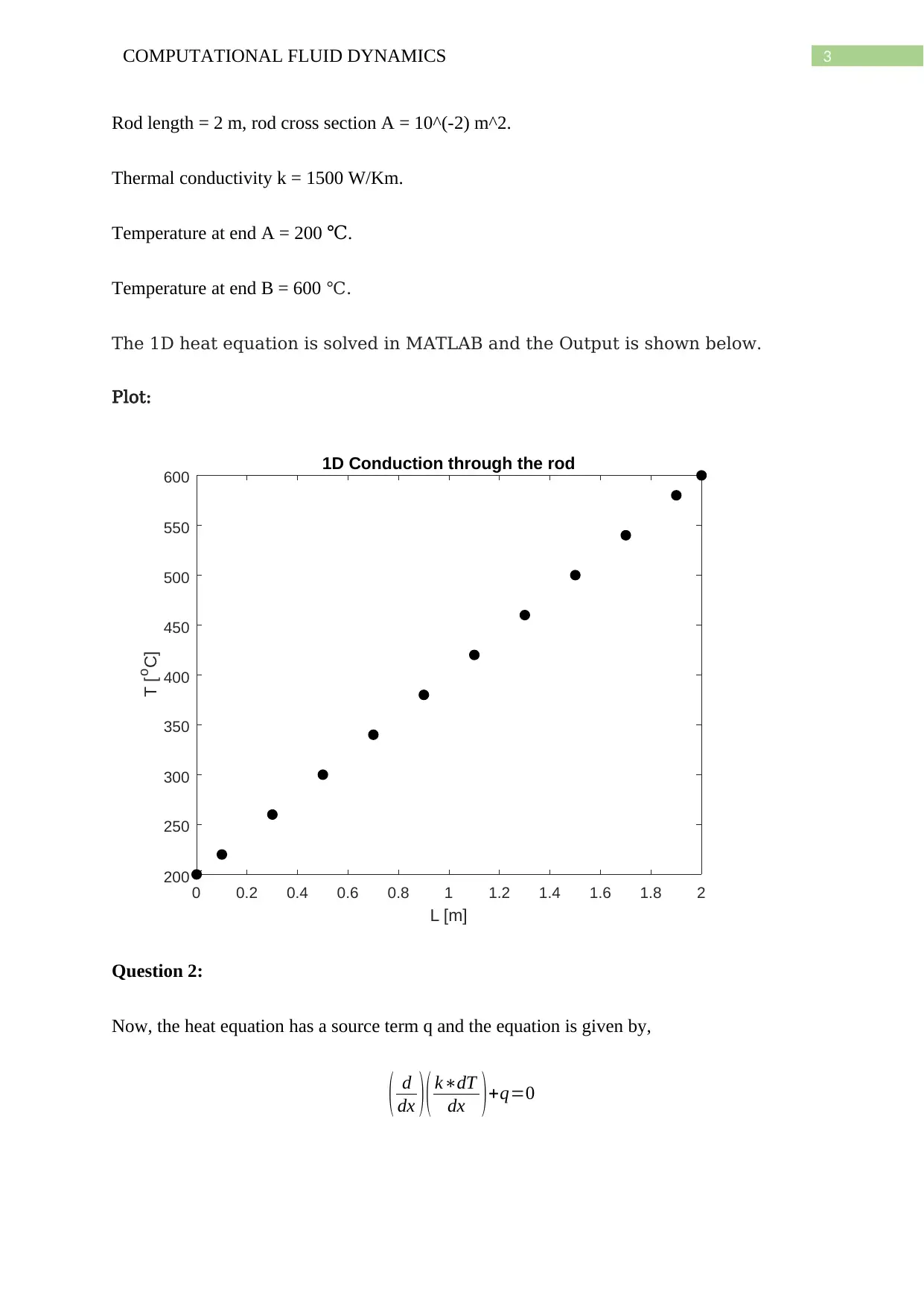
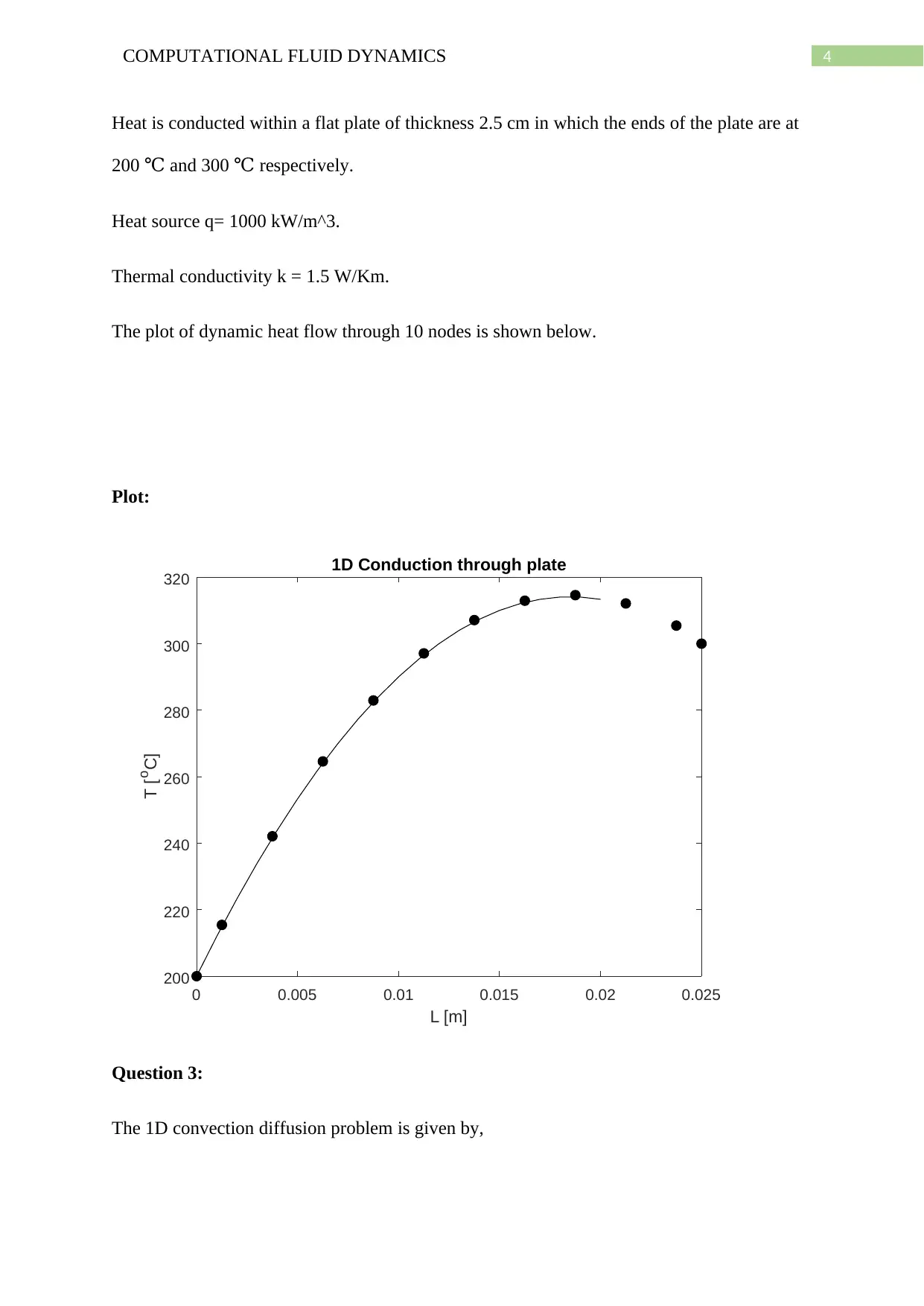
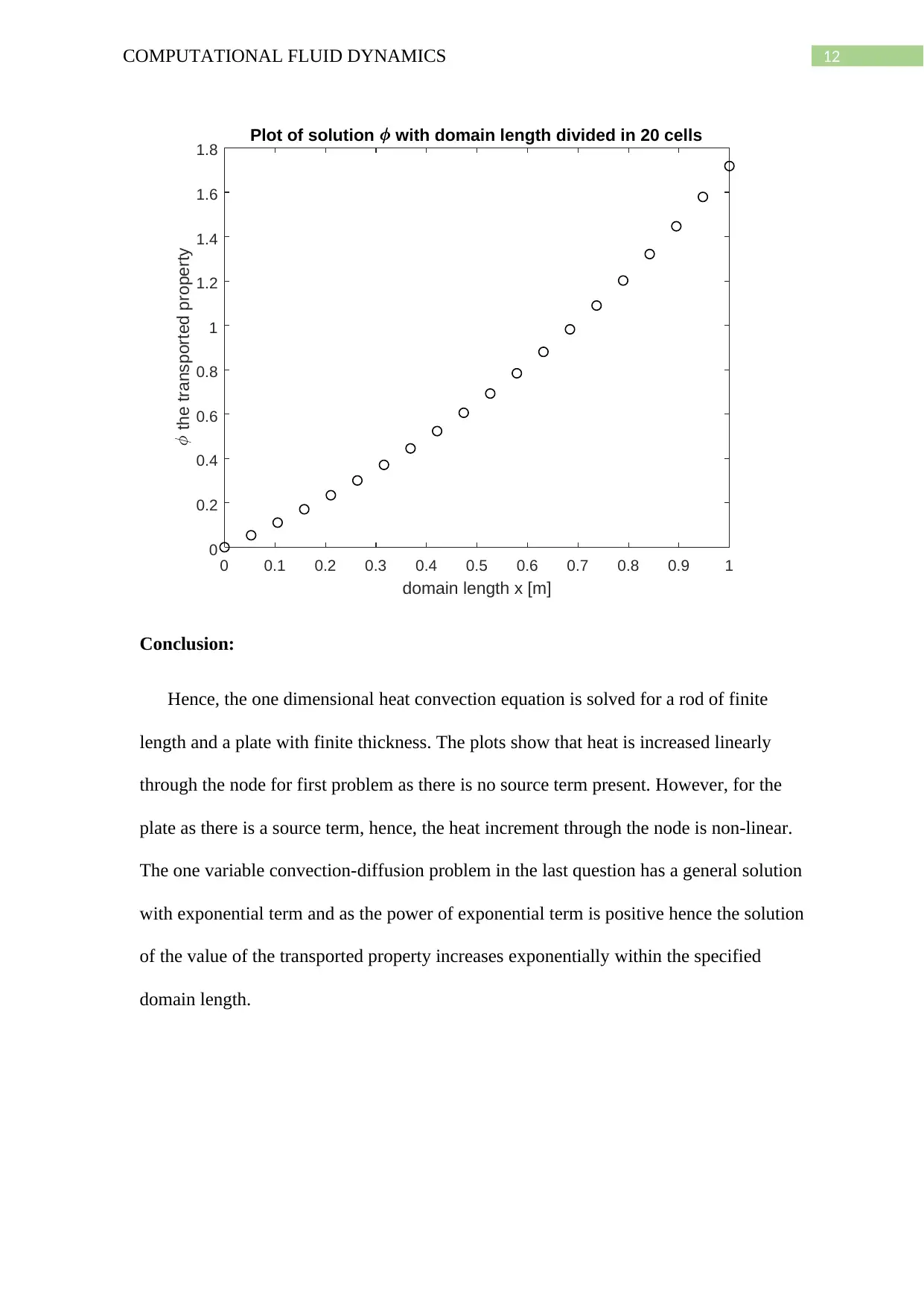
This project presents a computational fluid dynamics (CFD) analysis of 1D heat transfer problems. The finite volume method is employed to solve the heat conduction equation. The project is divided into three main parts. The first part investigates heat conduction through a rod with specified end temperatures, solved using MATLAB. The second part extends the analysis to a flat plate with a heat source term. The third part focuses on the convection-diffusion problem, solving it analytically and numerically using MATLAB for different convection speeds and cell numbers. The results are presented as plots, demonstrating the temperature distribution and the behavior of the transported property under various conditions. The project concludes with a discussion of the results and the influence of parameters on the heat transfer and convection-diffusion phenomena. The project showcases the application of CFD techniques for solving engineering problems related to heat transfer and fluid dynamics.

Running head: COMPUTATIONAL FLUID DYNAMICS
COMPUTATIONAL FLUID DYNAMICS
Name of the Student
Name of the University
Author Note

2COMPUTATIONAL FLUID DYNAMICS
Introduction:
The finite volume method is popularly used for solving heat conduction equation in 1
dimensional plane. Here, the general transport equation is discretized into several system of
linear equations. The linear equations are then solved using numerical methods or specifically
using Gauss-Siedel method and TDMA numerical method in MATLAB. The heat conduction
equation can be derived using the Energy balance equation in specific node. In the first
problem heat convection through a rod of 2 m is evaluated at different nodes where the end
temperatures are 200 °C and 600 °C respectively. In the second problem the heat convection
is evaluated for a plate of 2.5 cm, where, the two ends are maintained at temperatures 200 °C
and 600 °C. In the third problem the convection-diffusion problem is solved using Analytical
method and assuming suitable initial conditions for the property of interest. Generally, the
convection-diffusion has two variable the length x and time t and differential equation is
second order partial differential equation. However, in this case the problem is identified for
one variable, length x and the time variable t is assumed constant. Thus the convection-
diffusion equation becomes an ordinary differential equation of second order.
Question 1:
The 1D heat conduction equation is given by,
( d
dx )( k∗dT
dx )=0
Here, k is thermal conductivity.
T = local temperature
x = spatial co-ordinate
The dynamic temperature of the rod is found in 10 nodes.

3COMPUTATIONAL FLUID DYNAMICS
Rod length = 2 m, rod cross section A = 10^(-2) m^2.
Thermal conductivity k = 1500 W/Km.
Temperature at end A = 200 .℃
Temperature at end B = 600 ℃.
The 1D heat equation is solved in MATLAB and the Output is shown below.
Plot:
0 0.2 0.4 0.6 0.8 1 1.2 1.4 1.6 1.8 2
L [m]
200
250
300
350
400
450
500
550
600
T [oC]
1D Conduction through the rod
Question 2:
Now, the heat equation has a source term q and the equation is given by,
( d
dx )( k∗dT
dx )+q=0

4COMPUTATIONAL FLUID DYNAMICS
Heat is conducted within a flat plate of thickness 2.5 cm in which the ends of the plate are at
200 and 300 respectively.℃ ℃
Heat source q= 1000 kW/m^3.
Thermal conductivity k = 1.5 W/Km.
The plot of dynamic heat flow through 10 nodes is shown below.
Plot:
0 0.005 0.01 0.015 0.02 0.025
L [m]
200
220
240
260
280
300
320
T [oC]
1D Conduction through plate
Question 3:
The 1D convection diffusion problem is given by,

5COMPUTATIONAL FLUID DYNAMICS
( d
dx ) ( ρuϕ ) =( d
dx ) (Γ∗( dϕ
dx ))
ϕ =transported property
u = convection speed
Γ = diffusivity
ρ = density.
Domain length = 1 m.
Density ρ = 1 kg/m^3
Diffusivity Γ = 0.1 kg/ms.
i) Now, the convection speed u = 0.1 m/sec and the number of cells = 5 cells.
Here, the convection-diffusion problem has only one variable the domain length x in m in
[0,1].
Hence, putting the values in the equation (1) the convection-diffusion problem will be
( d
dx ) ( 0.1 ϕ ) =( d
dx ) ( 0.1∗( dϕ
dx ))
 0.1 d2 ϕ
d x2 – 0.1 dϕ
dx = 0
 d2 ϕ
d x2 - dϕ
dx = 0
The analytical solution of the equation is given by,
ϕ ( x )=c 1∗exp (x)+c 2
Where, c1 and c2 are constants.

6COMPUTATIONAL FLUID DYNAMICS
Now, when initial conditions are applied such that ϕ(0) = 0 and ˙ϕ(0) = 1 then the solution
becomes
ϕ ( x ) =exp ( x ) −1
Now, the solution is plotted in MATLAB by the following code.
MATLAB code:
u = 0.1; % convection speed in m/sec
gamma = 0.1; % diffusivity in kg/(m*sec)
rho = 1; % kg/m^3
% solving the differential equation
syms phi(x)
Dphi = diff(phi);
ode = (rho*u)*diff(phi,x,2) == gamma*diff(phi,x);
cond1 = phi(0) == 0;
cond2 = Dphi(0) == 1;
conds = [cond1 cond2];
phiSol(x) = dsolve(ode,conds)
n = 5; % number of cells

7COMPUTATIONAL FLUID DYNAMICS
L = 1; % domain length
x = linspace(0,L,n); % domain length of 1 m is divided in 5 cells
for i=1:length(x)
phisol(i) = eval(phiSol(x(i)));
end
plot(x,phisol,'ko')
title('Plot of solution phi with domain length divided in 5 cells')
xlabel('domain length x [m]')
ylabel('\phi the transported property')
Output:
phiSol(x) =
exp(x) - 1
Plot of solution ϕ (x ):

8COMPUTATIONAL FLUID DYNAMICS
0 0.1 0.2 0.3 0.4 0.5 0.6 0.7 0.8 0.9 1
domain length x [m]
0
0.2
0.4
0.6
0.8
1
1.2
1.4
1.6
1.8
the transported property
Plot of solution with domain length divided in 5 cells
ii) Now, the solution is plotted when u = 2.5 m/sec, cells = 5. All the initial conditions are
kept same as before.
MATLAB code:
u = 2.5; % convection speed in m/sec
gamma = 0.1; % diffusivity in kg/(m*sec)
rho = 1; % kg/m^3
% solving the differential equation
syms phi(x)
Dphi = diff(phi);

9COMPUTATIONAL FLUID DYNAMICS
ode = (rho*u)*diff(phi,x,2) == gamma*diff(phi,x);
cond1 = phi(0) == 0;
cond2 = Dphi(0) == 1;
conds = [cond1 cond2];
phiSol(x) = dsolve(ode,conds)
n = 5; % number of cells
L = 1; % domain length
x = linspace(0,L,n); % domain length of 1 m is divided in 5 cells
for i=1:length(x)
phisol(i) = eval(phiSol(x(i)));
end
plot(x,phisol,'ko')
title('Plot of solution phi with domain length divided in 5 cells')
xlabel('domain length x [m]')
ylabel('\phi the transported property')
Output:
phiSol(x) =
25*exp(x/25) – 25

10COMPUTATIONAL FLUID DYNAMICS
Plot:
0 0.1 0.2 0.3 0.4 0.5 0.6 0.7 0.8 0.9 1
domain length x [m]
0
0.2
0.4
0.6
0.8
1
1.2
the transported property
Plot of solution with domain length divided in 5 cells
iii) Now, convection speed u = 0.1 m/sec and cell numbers = 20. All the initial conditions
are kept same as before.
MATLAB code:
u = 0.1; % convection speed in m/sec
gamma = 0.1; % diffusivity in kg/(m*sec)
rho = 1; % kg/m^3
% solving the differential equation
syms phi(x)

11COMPUTATIONAL FLUID DYNAMICS
Dphi = diff(phi);
ode = (rho*u)*diff(phi,x,2) == gamma*diff(phi,x);
cond1 = phi(0) == 0;
cond2 = Dphi(0) == 1;
conds = [cond1 cond2];
phiSol(x) = dsolve(ode,conds)
n = 20; % number of cells
L = 1; % domain length
x = linspace(0,L,n); % domain length of 1 m is divided in 20 cells
for i=1:length(x)
phisol(i) = eval(phiSol(x(i)));
end
plot(x,phisol,'ko')
title('Plot of solution \phi with domain length divided in 20 cells')
xlabel('domain length x [m]')
ylabel('\phi the transported property')
Output:
phiSol(x) =
exp(x) - 1

12COMPUTATIONAL FLUID DYNAMICS
0 0.1 0.2 0.3 0.4 0.5 0.6 0.7 0.8 0.9 1
domain length x [m]
0
0.2
0.4
0.6
0.8
1
1.2
1.4
1.6
1.8
the transported property
Plot of solution with domain length divided in 20 cells
Conclusion:
Hence, the one dimensional heat convection equation is solved for a rod of finite
length and a plate with finite thickness. The plots show that heat is increased linearly
through the node for first problem as there is no source term present. However, for the
plate as there is a source term, hence, the heat increment through the node is non-linear.
The one variable convection-diffusion problem in the last question has a general solution
with exponential term and as the power of exponential term is positive hence the solution
of the value of the transported property increases exponentially within the specified
domain length.