Real World Analytics Project: Cooling Load Prediction and Optimization

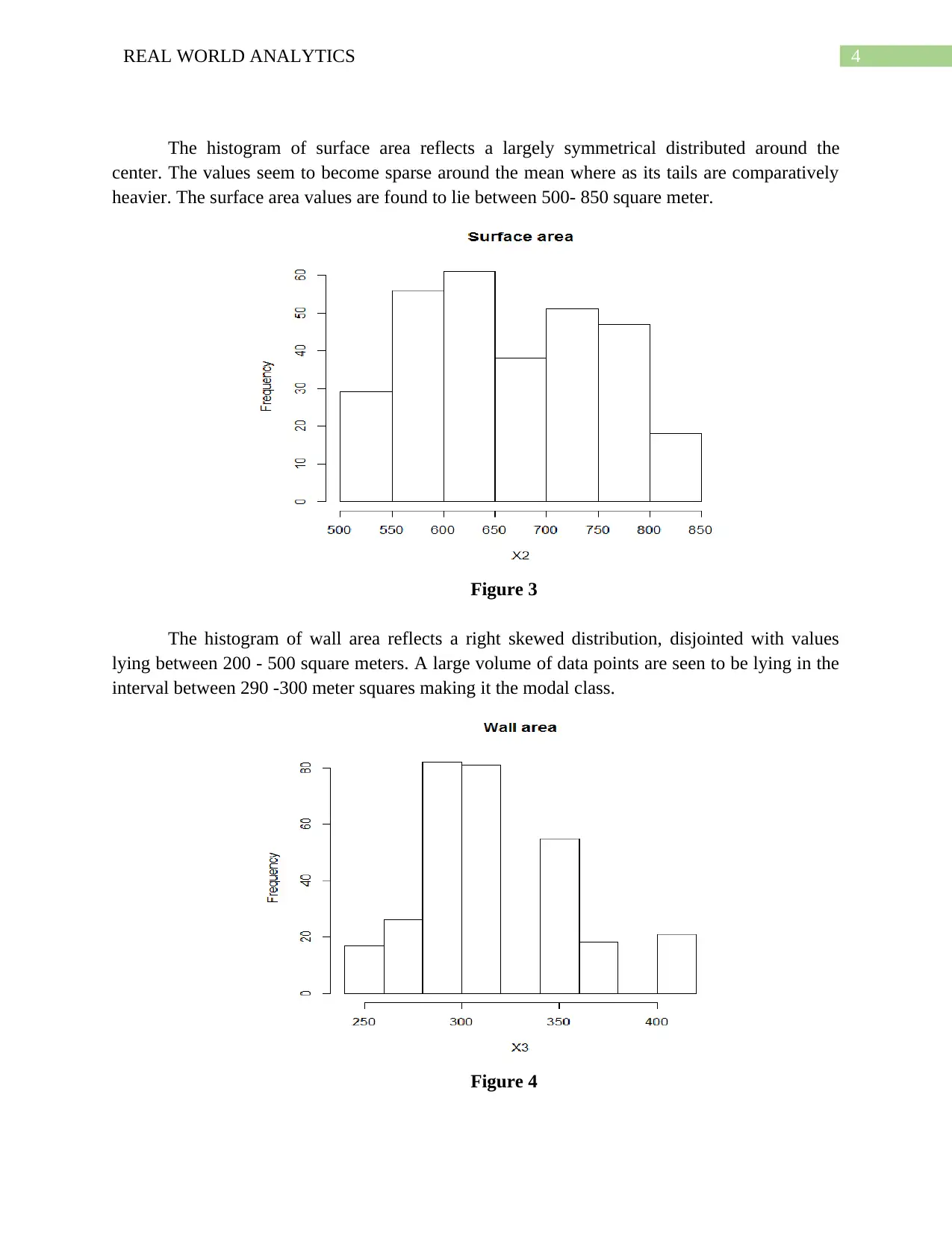
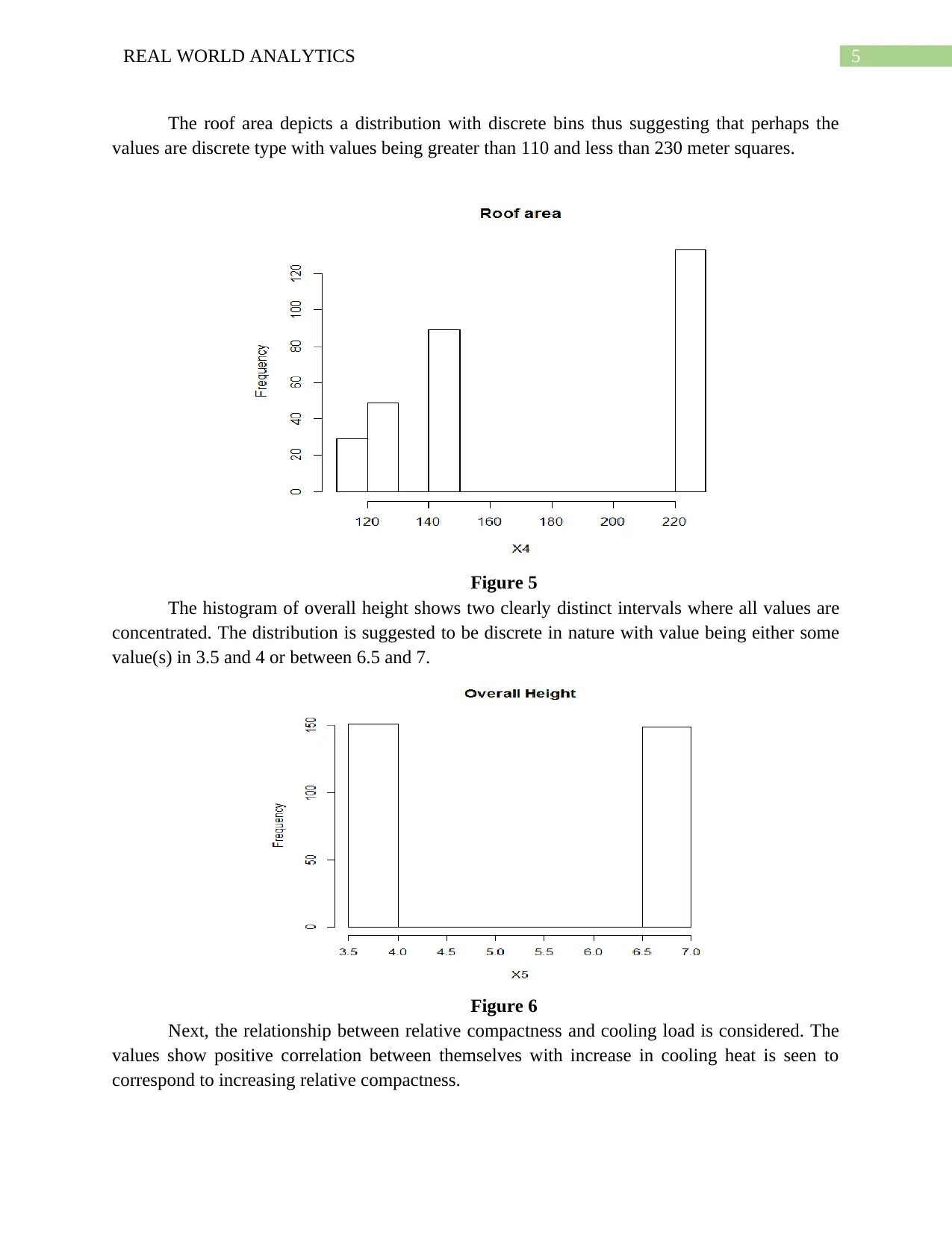
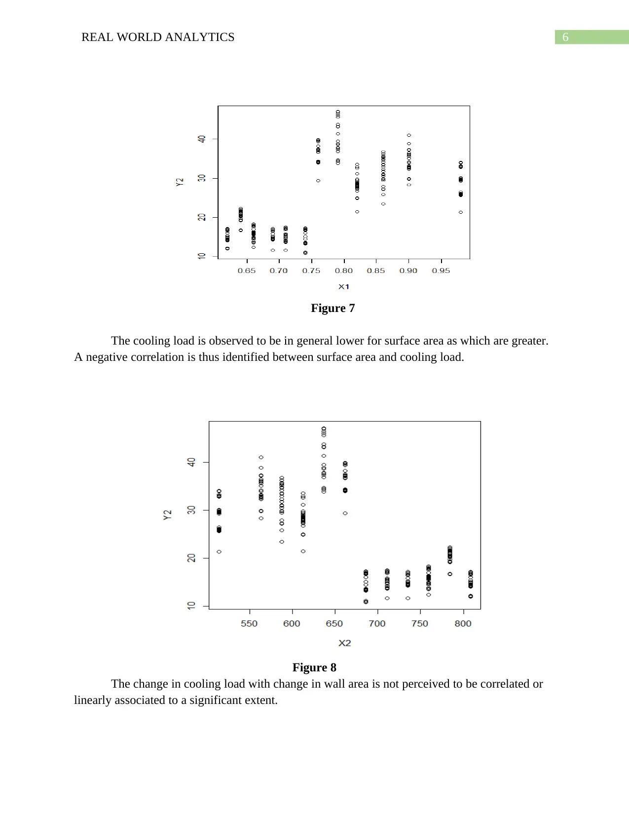
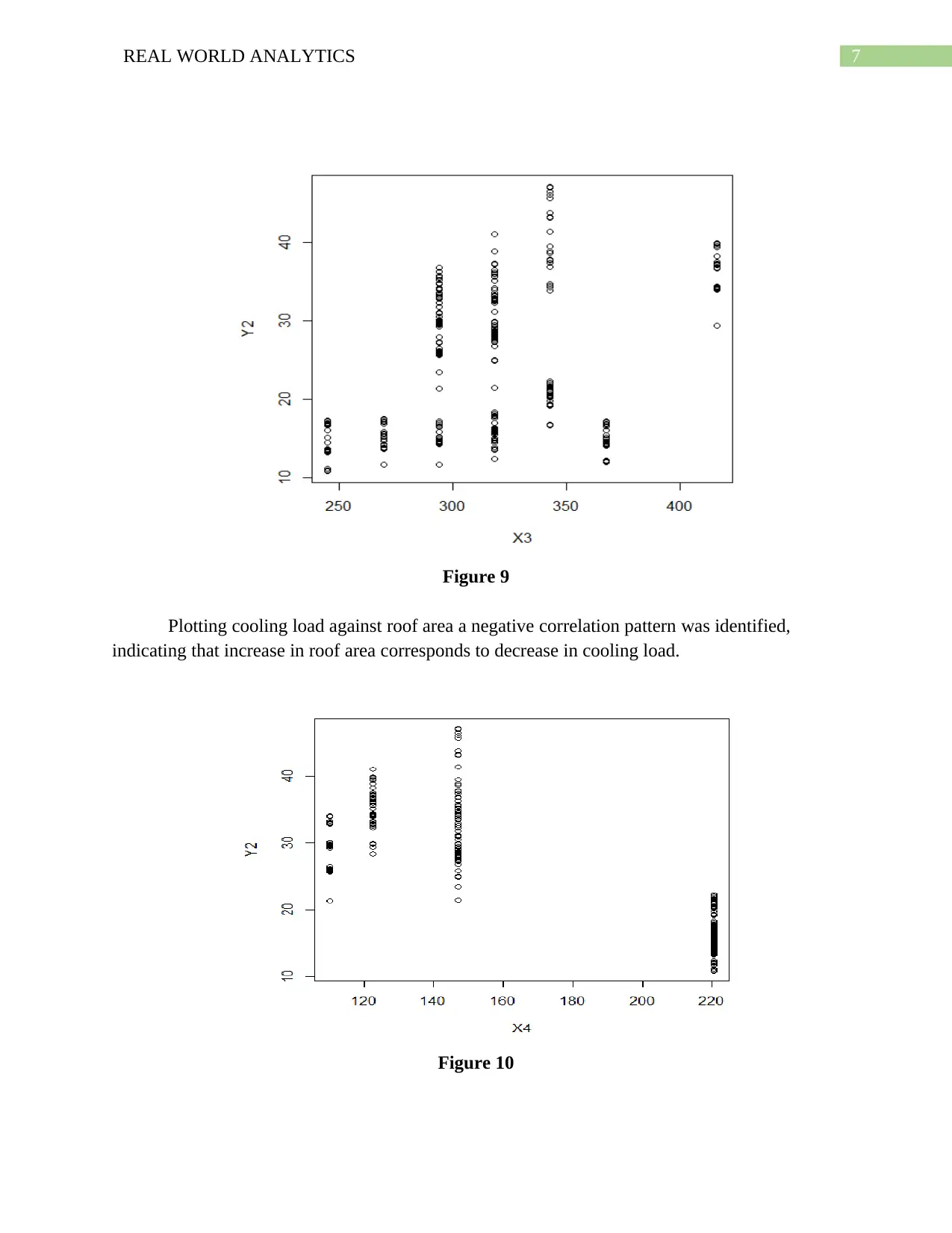
This project analyzes cooling load data to predict energy consumption in buildings. It utilizes a dataset of 300 samples, exploring the influence of various independent variables such as relative compactness, surface area, wall area, roof area, and overall height on cooling load. The analysis is conducted in R, involving data visualization through histograms and scatter plots to understand the relationships between variables. The project transforms variables to reduce skewness and employs different models, including weighted average mean, weighted power means, ordered weighted averages, and Choquet's integral, to predict cooling load. The weighted power average model with a power of 0.5 is identified as the best fit. Furthermore, a linear regression model is fitted, and the predicted cooling load is calculated based on specific values of the independent variables. Finally, the project extends to an optimization problem involving juice blending, defining constraints related to concentrate volumes to minimize the cost of the special juice.

Running head: REAL WORLD ANALYTICS
REAL WORLD ANALYTICS
Name of Student
Name of University

1REAL WORLD ANALYTICS
Table of Contents
Part A:..............................................................................................................................................2
Description...................................................................................................................................2
Task 1...........................................................................................................................................2
Task 2...........................................................................................................................................8
Task 3...........................................................................................................................................8
Task 4...........................................................................................................................................9
Part B.............................................................................................................................................10
1.................................................................................................................................................10

2REAL WORLD ANALYTICS
Part A:
Description
Heating load and cooling load serve to guide the specifications of equipment for heating
and cooling that are installed buildings. Therefore they are key variables to consider while
designing energy efficient buildings when considering how to optimize energy consumption.
The variables Heating load (Y1 or HL) and cooling load (Y2 or CL) are two variables
being considered to be of interest in this paper. The independent variables, viz., relative
compactness(X1) in percentage(in decimals),the surface area(X2) ,expressed in squared meter,
the wall area(X3) in square meter, the roof area(X4) in squared meter and finally the overall
height(X5) in meters are being considered as potential influences on the chosen response. The
analysis was done in R using a sample of size of 300.
Task 1
Following instructions, the data file ENB18data.txt was downloaded from CloudDeakin
into the R. Cooling Load or Y2 was selected as the variable of interest. The influence of the
variables X1, X2, X3, X4 and X5 on Y2 and their individual natures were analyzed on the basis
of the chosen sample and hence discussed.
The graphical descriptive summary of the variables and the relationships between the
cooling load and the variables X1, X2, X3, X4 and X5 are given as follows.
The histogram of the variable cooling load measured in the unit KWh per square meter
per annum is seen to have distribution which is skewed right with most values are seen to be
towards the left tail or the lower side of the X-axis making its left tail more steep and right tail
flatter and elongated than its left. The values lie between 10 to 50 KWh per square meter with
mode being between 15 - 20KWh per square meter.

3REAL WORLD ANALYTICS
Figure 1
The relative compactness values are observed to be between 0.6 and 1. The distribution is
positively or right skewed.
Figure 2

4REAL WORLD ANALYTICS
The histogram of surface area reflects a largely symmetrical distributed around the
center. The values seem to become sparse around the mean where as its tails are comparatively
heavier. The surface area values are found to lie between 500- 850 square meter.
Figure 3
The histogram of wall area reflects a right skewed distribution, disjointed with values
lying between 200 - 500 square meters. A large volume of data points are seen to be lying in the
interval between 290 -300 meter squares making it the modal class.
Figure 4

5REAL WORLD ANALYTICS
The roof area depicts a distribution with discrete bins thus suggesting that perhaps the
values are discrete type with values being greater than 110 and less than 230 meter squares.
Figure 5
The histogram of overall height shows two clearly distinct intervals where all values are
concentrated. The distribution is suggested to be discrete in nature with value being either some
value(s) in 3.5 and 4 or between 6.5 and 7.
Figure 6
Next, the relationship between relative compactness and cooling load is considered. The
values show positive correlation between themselves with increase in cooling heat is seen to
correspond to increasing relative compactness.

6REAL WORLD ANALYTICS
Figure 7
The cooling load is observed to be in general lower for surface area as which are greater.
A negative correlation is thus identified between surface area and cooling load.
Figure 8
The change in cooling load with change in wall area is not perceived to be correlated or
linearly associated to a significant extent.

7REAL WORLD ANALYTICS
Figure 9
Plotting cooling load against roof area a negative correlation pattern was identified,
indicating that increase in roof area corresponds to decrease in cooling load.
Figure 10

8REAL WORLD ANALYTICS
Plotting cooling load against overall height a positive linear relationship was indicated
whereby, increase in overall height corresponded to higher cooling load values. The height was
suspected to be discrete and two distinct clusters of cooling load could be identified from the
scatter plot.
Figure 11
Task 2
Four variables out of the five independent variables that were selected for the purpose of
predicting cooling load with the exception of X3 or wall area which failed to show significant relationship
with the cooling lead. The data were saved in a data file labelled “name-transformed.txt”. The variables
were further transformed to decrease the skewness by taking logarithm of the variables. It is to be noted
that the general relationship between the variables do not change significantly even after transformation.
Task 3
Parameters for the WAM or weighted average mean, PMs or weighted power averages with
power 0.5 and 2, ordered weighted means and Choquet’s integral were important.
The following tables give the parameters and summary of the fit for the four models:
Model RMSE Av. abs.
error
Pearson’s
Correlation
Spearman’s
Correlation
Weighted Average 7.549 6.4860 0.7436 0.81513
Weighted Power mean
(P=0.05)
6.60415 5.3515 0.8808 0.8761
Weighted power mean
(P=2)
8.711 7.513 0.5032 0.5333
Ordered weighted
average
7.5489 6.4860 0.74360 0.81513

9REAL WORLD ANALYTICS
Choquet’s Integral 7.5489 6.4860 0.74360 0.80521
Table 1: Error measures and correlation
Variable Weighted
Average
Weighted
Power
P=0.05
Weighted
power
P=2
Ordered
weighted
average
Choquet’s
Integral
X1 0 0 0 0 0
X2 0 0 0 0.934 0
X3 0.0657 0.165 0.007 0 0.032
X4 0 0 0 0.065 0.032
X5 0.9342 0.834 0.9929 0 0.9342
Table 2: Model Parameters
The weighted power average model with the parameter power being 0.5 was found to have the
least value of RMSE and average absolute error among all other models. Additionally it had higher
correlation coefficient values than others. Thus this was considered as the best model. Wall area and
overall height were identified as the variables with most weightage by the model. Furthermore, higher
values of these variables, was specified to account for greater values of cooling load.
Task 4
The four variable identified, transformed to their respective logarithm counterparts and saved in
the text file “name-transformed.txt”, were used to fit a linear regression to predict the transformed
logarithm of Y2 variable. However only X1, X2 and X5 were found to have significant effects so the
model with relative compactness, surface area and overall height to predict Y2 was considered to have the
better fit. Using the values specified as X1 equals 0.82, X2 equals 612.5, X3 being 318.5, X4 being 147
and X5 being 7, the predicted value of the logarithm of Y2 was found to be 3.50 and hence predicted Y2
was 33.312. Greater values of X1, X2, and X5 correspond with higher Y2.

10REAL WORLD ANALYTICS
Part B
1.
(a)
The problem dictates that a special juice is to be concocted using two juices A and B. Let
X1 be the volume of Juice A and X2 be the volume of juice B. The problem states that there has to be at
the least 3.5 litres of Orange concentrate per 100 litres , at least 4 litres of Apple concentrate per 100 litres
of the Juice in the special juice respectively. However it is also specified that no more than 6 litres of
Carrot concentrate per 100 litres should be present. Thus the constraints for carrot concentrate can be
written as:
“4X1+8X2<=6”. Again, that for oranges it can be written as “6X1+3X2>=3.5” and that for apples it can
be written as “3X1+6X2>=4”. The customer had also specified that at least 50 litres of the juice would be
required per week, thus another constraint is to be considered, which is, “X1+X2>=50”. Additionally,
there also are the non-negativity constraints, “X1>=0” and “X2>=0”. Given all these above constraints,
the problem is to minimize the cost of making the special juice. Thus since cost of Juice A is $6 and that
of juice B is $5, and they are fixed, the amount of juice X1 and X2 is to be determined which can
minimize the cost function which is “F=6X1+5X2” subject to the constraints mentioned above.