Cooling Tank Control: Modeling, Simulation, and Control Design
VerifiedAdded on 2023/06/03
|24
|4900
|69
Project
AI Summary
This project focuses on the design and analysis of a cooling tank control system. The assignment begins with an introduction and problem statement, followed by a detailed explanation of the system parameters and assumptions. It then delves into the cooling tank controller design tasks, which include steady-state balance equations, energy balance equations, and transfer function derivation. The project continues with the development of a Simulink model for the system and the creation of linear deviation models. Furthermore, the assignment explores the reaction rate, Arrhenius temperature dependence, and the application of a PID controller. The project utilizes MATLAB to plot the reaction curve and determine the controller parameters, providing a comprehensive understanding of cooling tank control system design and implementation.
COOLING TANK CONTROL
ASSIGNMENT
INSTITUTIONAL AFFILIATION
LOCATION
INSTRUCTOR (PROFESSOR)
STUDENT NAME
STUDENT ID NUMBER
DATE OF SUBMISSION
1
ASSIGNMENT
INSTITUTIONAL AFFILIATION
LOCATION
INSTRUCTOR (PROFESSOR)
STUDENT NAME
STUDENT ID NUMBER
DATE OF SUBMISSION
1
Paraphrase This Document
Need a fresh take? Get an instant paraphrase of this document with our AI Paraphraser
TABLE OF CONTENTS
INTRODUCTION...........................................................................................................................2
PROBLEM STATEMENT..........................................................................................................2
ASSUMPTIONS..........................................................................................................................2
SYSTEM PARAMETERS..........................................................................................................2
COOLING TANK CONTROLLER DESIGN TASKS..................................................................3
PART I.........................................................................................................................................3
PART II........................................................................................................................................9
PART III....................................................................................................................................10
PART IV....................................................................................................................................12
PART V......................................................................................................................................15
PART VI....................................................................................................................................16
DISCUSSION................................................................................................................................17
Process modeling.......................................................................................................................17
Control systems..........................................................................................................................19
Heat transfer in Thermodynamics..............................................................................................21
CONCLUSION..............................................................................................................................22
2
INTRODUCTION
PROBLEM STATEMENT
A hot liquid flow is coming to the tank with flow rate F and temperature T0. The liquid in
the tank is cooled by a jacket cooling water with flow rate Fc and inlet temperature Tcin. The
outlet temperature of cooling water is Tcout. By controlling the jacket cooling water flow rate, the
outlet temperature of the tank, T, can be maintained at a desired level.
ASSUMPTIONS
(i) The cooling tank is properly insulated to avoid heat transfer to the surroundings.
(ii) The amassing of energy in the tank walls and cooling jacket is considered negligible
compared to the accumulation of energy in the liquid.
(iii) It the liquid in the tank is well-mixed and the system is initially at steady state and the
physical properties of the liquid and tank environment are constant.
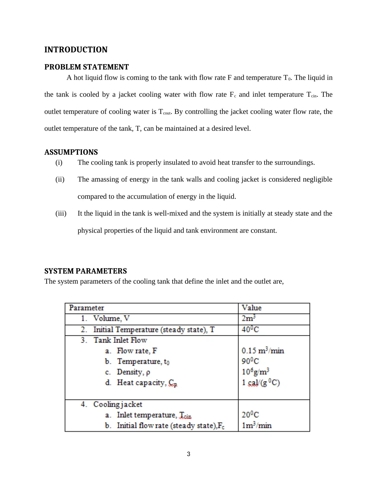
SYSTEM PARAMETERS
The system parameters of the cooling tank that define the inlet and the outlet are,
3
PROBLEM STATEMENT
A hot liquid flow is coming to the tank with flow rate F and temperature T0. The liquid in
the tank is cooled by a jacket cooling water with flow rate Fc and inlet temperature Tcin. The
outlet temperature of cooling water is Tcout. By controlling the jacket cooling water flow rate, the
outlet temperature of the tank, T, can be maintained at a desired level.
ASSUMPTIONS
(i) The cooling tank is properly insulated to avoid heat transfer to the surroundings.
(ii) The amassing of energy in the tank walls and cooling jacket is considered negligible
compared to the accumulation of energy in the liquid.
(iii) It the liquid in the tank is well-mixed and the system is initially at steady state and the
physical properties of the liquid and tank environment are constant.
SYSTEM PARAMETERS
The system parameters of the cooling tank that define the inlet and the outlet are,
3
⊘ This is a preview!⊘
Do you want full access?
Subscribe today to unlock all pages.
Trusted by 1+ million students worldwide
COOLING TANK CONTROLLER DESIGN TASKS
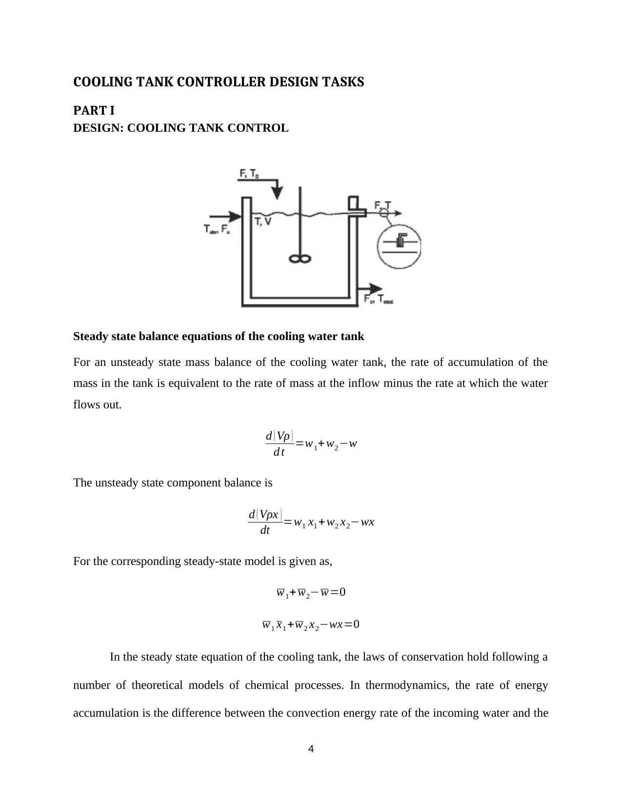
PART I
DESIGN: COOLING TANK CONTROL
Steady state balance equations of the cooling water tank
For an unsteady state mass balance of the cooling water tank, the rate of accumulation of the
mass in the tank is equivalent to the rate of mass at the inflow minus the rate at which the water
flows out.
d ( Vρ )
d t =w1+ w2 −w
The unsteady state component balance is
d ( Vρx )
dt =w1 x1 + w2 x2−wx
For the corresponding steady-state model is given as,
w1+w2−w=0
w1 x1 +w2 x2−wx=0
In the steady state equation of the cooling tank, the laws of conservation hold following a
number of theoretical models of chemical processes. In thermodynamics, the rate of energy
accumulation is the difference between the convection energy rate of the incoming water and the
4
Paraphrase This Document
Need a fresh take? Get an instant paraphrase of this document with our AI Paraphraser
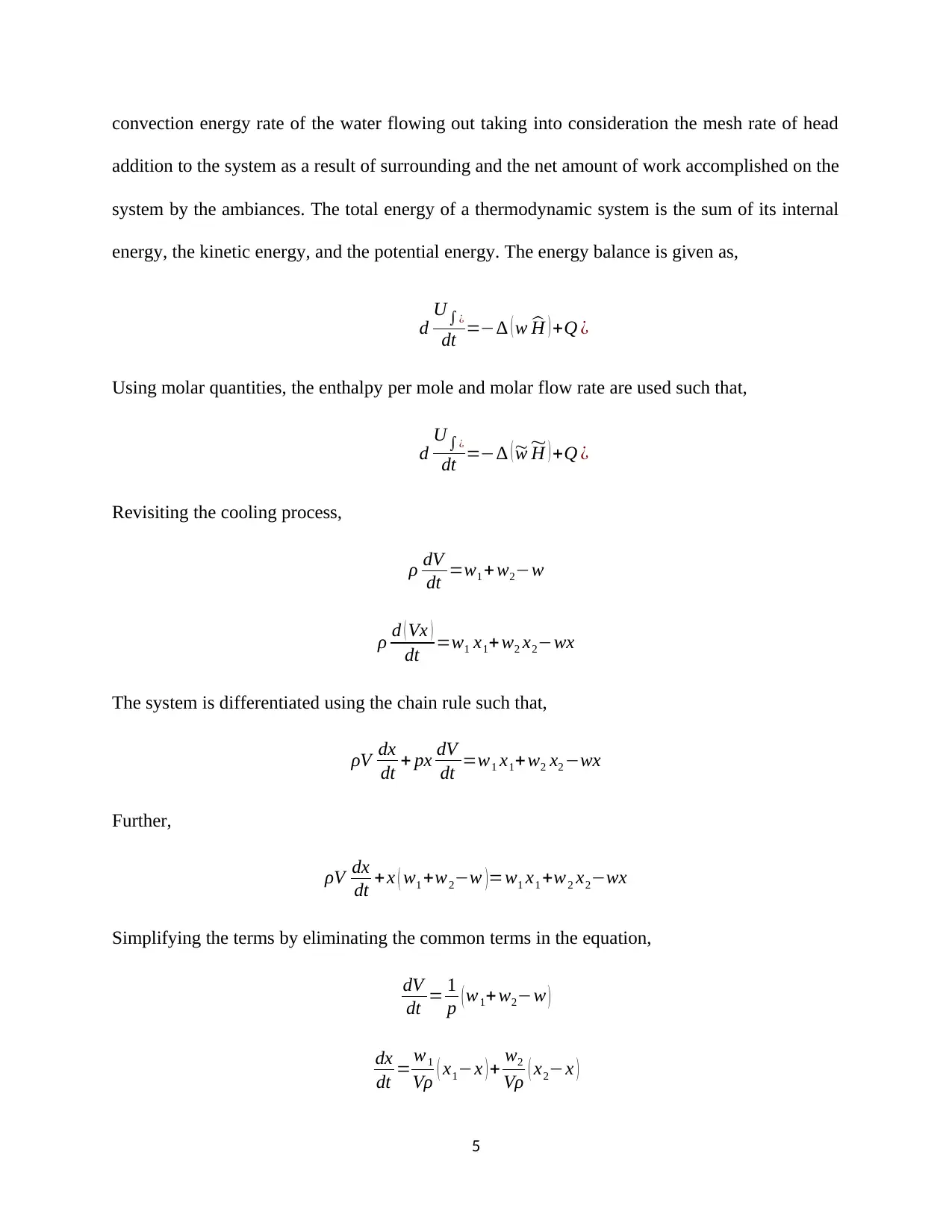
convection energy rate of the water flowing out taking into consideration the mesh rate of head
addition to the system as a result of surrounding and the net amount of work accomplished on the
system by the ambiances. The total energy of a thermodynamic system is the sum of its internal
energy, the kinetic energy, and the potential energy. The energy balance is given as,
d U∫¿
dt =−∆ ( w ^H ) +Q ¿
Using molar quantities, the enthalpy per mole and molar flow rate are used such that,
d U∫¿
dt =−∆ ( ~w ~
H ) +Q ¿
Revisiting the cooling process,
ρ dV
dt =w1 + w2−w
ρ d ( Vx )
dt =w1 x1+ w2 x2−wx
The system is differentiated using the chain rule such that,
ρV dx
dt + px dV
dt =w1 x1+w2 x2 −wx
Further,
ρV dx
dt + x ( w1 +w2−w )=w1 x1 +w2 x2−wx
Simplifying the terms by eliminating the common terms in the equation,
dV
dt = 1
p ( w1+ w2−w )
dx
dt = w1
Vρ ( x1−x ) + w2
Vρ ( x2−x )
5

In the cooling tank scenario, it is possible to determine the amassing of the internal energy such
that,
d U∫¿
dt =ρVC dT
dt ¿
For the cooling tank with a temperature T with an enthalpy H,
^H− ^H ref =C ( T −T ref )
^Href =0
^H=C ( T −T ref )
At the inlet valve section,
^Hi=C ( Ti −Tref )
The convection energy is given as,
−∆ ( w ^H ) =w [ C ( T i−T ref ) ] −w [ c ( T −T ref ) ]
VρC dT
dt =wC ( Ti−T ) +Q
At the outlet valve section,
^Hout =C ( T out−T ref )
The convection energy is given as,
−∆ ( w ^Hout )=w [ C (T out−T ref ) ]−w [ c ( Tout −Tref ) ]
6
⊘ This is a preview!⊘
Do you want full access?
Subscribe today to unlock all pages.
Trusted by 1+ million students worldwide
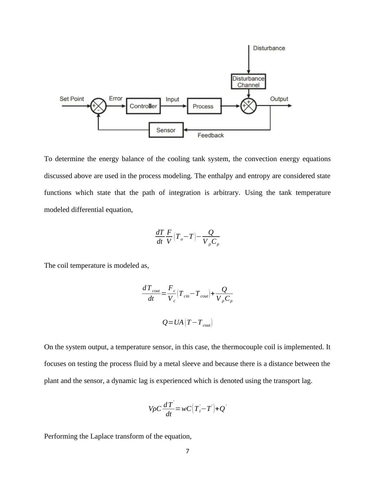
To determine the energy balance of the cooling tank system, the convection energy equations
discussed above are used in the process modeling. The enthalpy and entropy are considered state
functions which state that the path of integration is arbitrary. Using the tank temperature
modeled differential equation,
dT
dt
F
V ( T o−T )− Q
V ρ Cρ
The coil temperature is modeled as,
d T cout
dt = Fc
V c
( T cin−T cout ) + Q
V ρ Cρ
Q=UA ( T −T cout )
On the system output, a temperature sensor, in this case, the thermocouple coil is implemented. It
focuses on testing the process fluid by a metal sleeve and because there is a distance between the
plant and the sensor, a dynamic lag is experienced which is denoted using the transport lag.
VρC d T '
dt =wC ( T i
' −T' )+Q'
Performing the Laplace transform of the equation,
7
Paraphrase This Document
Need a fresh take? Get an instant paraphrase of this document with our AI Paraphraser
VρC [ s T ' ( s ) −T ' ( 0 ) ] =wC [ T i
' ( s ) −T' ( s ) ] −Q' ( s )
For the initial steady state, T ' ( 0 ) =0
VρC [ s T ' ( s ) ] =wC [ T i
' ( s ) −T ' ( s ) ] −Q' ( s )
Rearranging the terms in the equation,
T ' ( s )= [ K
τs+1 ]Q' ( s ) +
[ 1
τs+1 ]Ti
' ( s )
K= 1
wC
τ =Vρ
w
T ' ( s )=G1 ( s ) Q' ( s ) +G2 ( s ) T i
' ( s)
The steady state of a transfer function is used in the calculation of the change in the steady state
value at the input. In a linear system, K is constant and for the nonlinear system, K depends on
the operating condition (Gene, J. Davied, & Abbas, 2010). The steady state gain is expressed
using the final value theorem such that,
K=lim
s →0
G( s)
G ( s )= Y ( s )
U ( s ) =
∑
i=0
m
bi si
∑
i=0
n
ai si
8
When the sensor is placed at the temperature downstream from the heated tank with a reasonable
transport lag, the distance L is used in the plug flow. The dead time is given as,
θ= L
V
The tank’s transfer function is given as,
G1= T ( s )
U ( s ) = K1
1+τ1 s
The sensor is given as,
G2= T cout ( s )
Tcin ( s ) = K2 e−θs
1+τ2 s K2 ≤ 1
Neglecting the value of τ 2, the overall transfer function is given as,
Tcou t ( s )
U =G2 . G1= K 1 K2 e−θs
1+τ1 s
Replacing with actual values,
0= F'
V (T o
' −T ' )− Q'
V ρ Cp
Q'=ρ C p F' ( T o
' −T' )
Q'= ( 0.15 x ( 90−40 ) x 106 x 1 )
Q '=7.5 x 10⁶ cal/min
0= F ❑c '
V❑c
(T cin
' −T cout
' )+ Q'
V ❑c ρc C p
T cout
' = V ❑c
F ❑c '∗
( Tcin
'
V ❑c
+ Q'
V ❑c
ρc C p )
9
⊘ This is a preview!⊘
Do you want full access?
Subscribe today to unlock all pages.
Trusted by 1+ million students worldwide
T cout
' = 0.5
1 ∗¿
T cout=27. 50 C
UA= Q
( T −T cout )
UA=7.5 x 10⁶
40−27.5
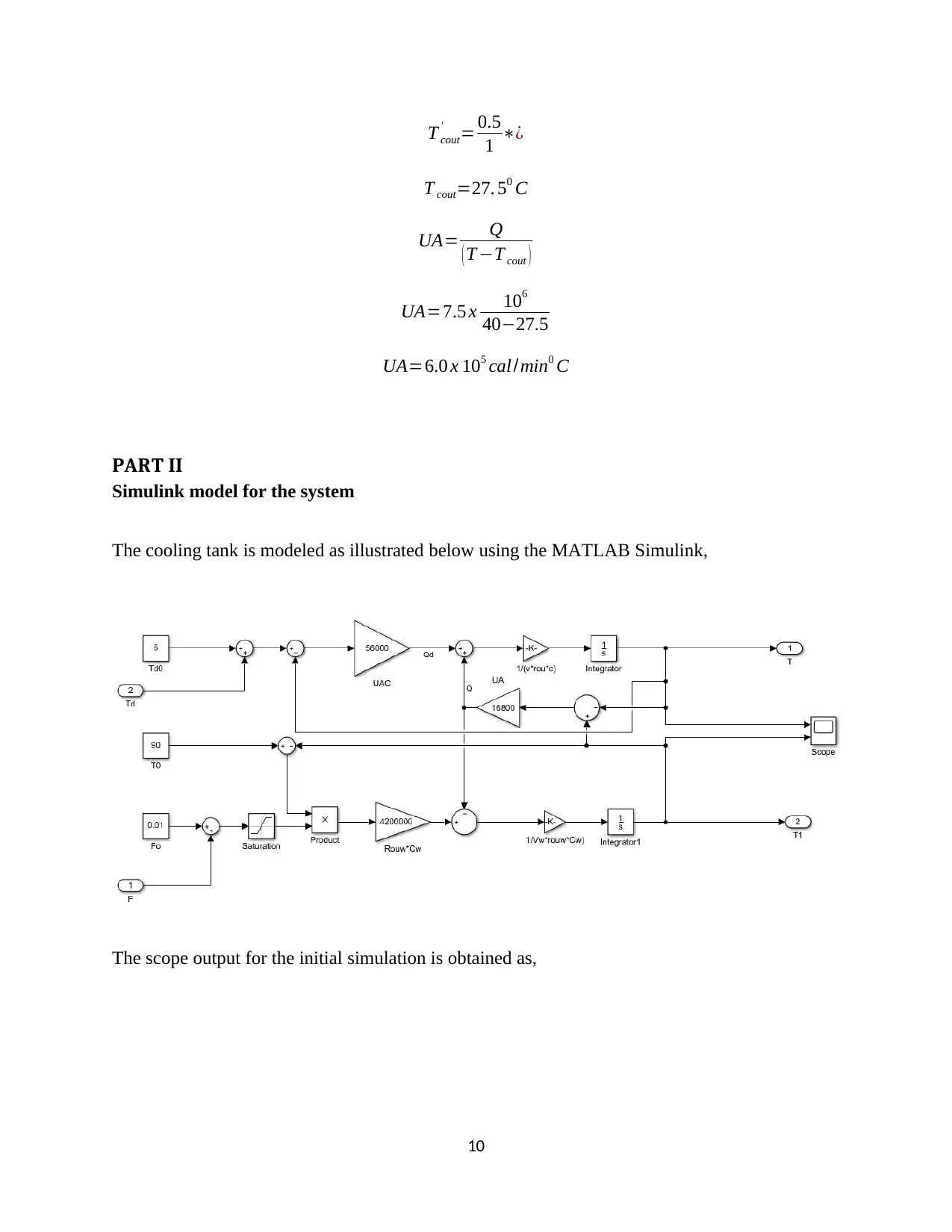
UA=6.0 x 10⁵ cal /min0 C
PART II
Simulink model for the system
The cooling tank is modeled as illustrated below using the MATLAB Simulink,
The scope output for the initial simulation is obtained as,
10
' = 0.5
1 ∗¿
T cout=27. 50 C
UA= Q
( T −T cout )
UA=7.5 x 10⁶
40−27.5
UA=6.0 x 10⁵ cal /min0 C
PART II
Simulink model for the system
The cooling tank is modeled as illustrated below using the MATLAB Simulink,
The scope output for the initial simulation is obtained as,
10
Paraphrase This Document
Need a fresh take? Get an instant paraphrase of this document with our AI Paraphraser
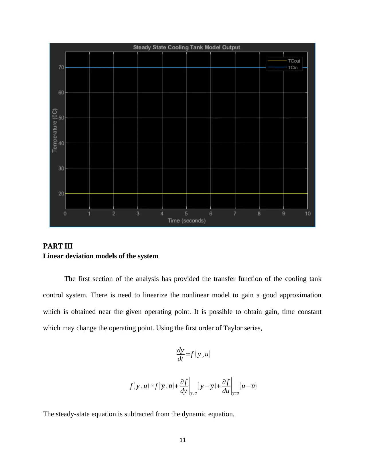
PART III
Linear deviation models of the system
The first section of the analysis has provided the transfer function of the cooling tank
control system. There is need to linearize the nonlinear model to gain a good approximation
which is obtained near the given operating point. It is possible to obtain gain, time constant
which may change the operating point. Using the first order of Taylor series,
dy
dt =f ( y , u )
f ( y , u ) ≅ f ( y , u ) + ∂ f
dy |y ,u
( y− y ) + ∂ f
du |y ,u
( u−u )
The steady-state equation is subtracted from the dynamic equation,
11
d y'
dt = ∂ f
dy |s
y'+ ∂ f
du |s
u'
The control and disturbance parameters are used to assess the linear time variables,
As H' ( s ) =qi
' ( s ) −q0
' ( s ) … deviation variables
The control variable is constant, hence, q0
' =0
As H' ( s )=qi
' ( s ) , H' ( s )
qi
' ( s ) = 1
As
The pure integrator in ramp form is used to obtain the step change in qi. The control variable is
given as shown for the non-linear element,
q0=Cv √h
The linear model is given as,
q'= 1
R h'
A d h'
dt =qi
' − 1
R h'
If q0=Cv √h
A d h'
dt =qi
'−Cv √ h
Performing Taylor series on the right hand side of the equation,
A d h'
dt =qi
' −Cv h0.5+ ∂ f
d qi
( qi−qi ) + ∂ f
dh ( h−h )
A d h'
dt =0+ ( qi −qi ) −1
2 Cv h−0.5 ( h−h )
qi
' − 1
2 Cv h−0.5 h'
A d h'
dt =qi
' − 1
R h'
12
⊘ This is a preview!⊘
Do you want full access?
Subscribe today to unlock all pages.
Trusted by 1+ million students worldwide
1 out of 24

Your All-in-One AI-Powered Toolkit for Academic Success.
+13062052269
info@desklib.com
Available 24*7 on WhatsApp / Email
![[object Object]](/_next/static/media/star-bottom.7253800d.svg)
Unlock your academic potential
Copyright © 2020–2026 A2Z Services. All Rights Reserved. Developed and managed by ZUCOL.